2.1 Oxford Flower VLAD and Fisher Vector Retrieval Demo

This notebook demonstrates how to:

1. Load the Oxford Flower dataset.

2. Extract deep convolutional features (last conv layer) from the resnet18 model.

3. Train a VLAD model on these deep features.

4. Perform image retrieval queries.

5. Show the effect of PCA (reducing features by half before VLAD) on retrieval performance.

6. An analogous procedure is made for Fisher Vectors

References

[1] Relja Arandjelović and Andrew Zisserman, ‘All About VLAD’, Department of Engineering Science, University of Oxford.
[2] Liangliang Wang and Deepu Rajan, “An Image Similarity Descriptor for Classification Tasks,” J. Vis. Commun. Image R., vol. 71, pp. 102847, 2020.

1. Imports and Setup

import os
from collections.abc import Sequence

import matplotlib.pyplot as plt
import numpy as np
import torch
from PIL import Image

from pyvisim.classic import FisherVectorEmbedder, VLADEmbedder
from pyvisim.datasets import OxfordFlowerDataset

# Our library imports
from pyvisim.neural_networks.features import DeepConvFeature
from pyvisim.retrieval.data import Candidate
from pyvisim.retrieval.image_store import InMemoryImageEmbeddingStore
from pyvisim.typing import UInt8NumpyArray

/home/runner/work/Python-Visual-Similarity/Python-Visual-Similarity/.venv/lib/python3.10/site-packages/tqdm/auto.py:21: TqdmWarning: IProgress not found. Please update jupyter and ipywidgets. See https://ipywidgets.readthedocs.io/en/stable/user_install.html
  from .autonotebook import tqdm as notebook_tqdm

Hyperparameters

Note

• Training k-means models takes quite a bit of time. In this notebook, a single n_clusters = 32 will be used. Change NUM_CLUSTERS to experiment with different cluster sizes.

• IMAGE_STEP keeps every IMAGE_STEP-th training image, both to train the embedders and to build the image stores. Set to 1 if you want to use all images.

NUM_CLUSTERS = 32
DIM_REDUCTION_FACTOR = 2
IMAGE_STEP = 4

Helper functions

def plot_image(image: UInt8NumpyArray | torch.Tensor, title: str = "Image") -> None:
    """
    Plot a single image.

    :param image: Image as a NumPy array (H, W, C) or torch tensor (C, H, W)
    :param title: Title of the plot
    """
    plt.figure(figsize=(10, 10))
    if isinstance(image, torch.Tensor):
        image = image.detach().cpu()
        if image.ndim == 3:
            image = image.permute(1, 2, 0)
        image = image.numpy()
    plt.imshow(image)
    plt.axis("off")
    plt.title(title)
    plt.show()


def plot_candidates(
    query_image: UInt8NumpyArray,
    query_label: int,
    candidates: Sequence[Candidate],
    labels_by_path: dict[str, int],
) -> None:
    """
    Plot a query image next to the gallery images retrieved for it.

    :param query_image: Query image as a NumPy array (H, W, C)
    :param query_label: Class label of the query image
    :param candidates: Ranked candidates retrieved for the query, e.g. by
        :meth:`~pyvisim.retrieval.image_store.InMemoryImageEmbeddingStore.retrieve_top_k_similar`
    :param labels_by_path: Class label of every gallery image, keyed by its path
    :raises KeyError: If a candidate path is missing from ``labels_by_path``
    """
    num_plots = len(candidates) + 1
    _, axes = plt.subplots(1, num_plots, figsize=(4 * num_plots, 4), squeeze=False)
    axes[0, 0].imshow(query_image)
    axes[0, 0].set_title(f"Query image. Label: {query_label}")
    for axis, candidate in zip(axes[0, 1:], candidates, strict=True):
        axis.imshow(_read_rgb_image(candidate.path))
        axis.set_title(
            f"Retrieved image. Label: {labels_by_path[candidate.path]}\n"
            f"Score: {candidate.score:.4f}"
        )
    for axis in axes[0]:
        axis.axis("off")
    plt.show()


def _read_rgb_image(path: str) -> UInt8NumpyArray:
    """
    Read an image file into an RGB array.

    :param path: Path to the image file
    :return: The image as a NumPy array (H, W, 3)
    """
    with Image.open(path) as image:
        return np.asarray(image.convert("RGB"))

2. Declare the Oxford Flower Dataset

train_dataset = OxfordFlowerDataset(purpose="train")
val_dataset = OxfordFlowerDataset(purpose="validation")
print("Number of images in the dataset:", len(train_dataset))

train_indices = range(0, len(train_dataset), IMAGE_STEP)
print("Number of images used for training and retrieval:", len(train_indices))

Number of images in the dataset: 6149
Number of images used for training and retrieval: 1538

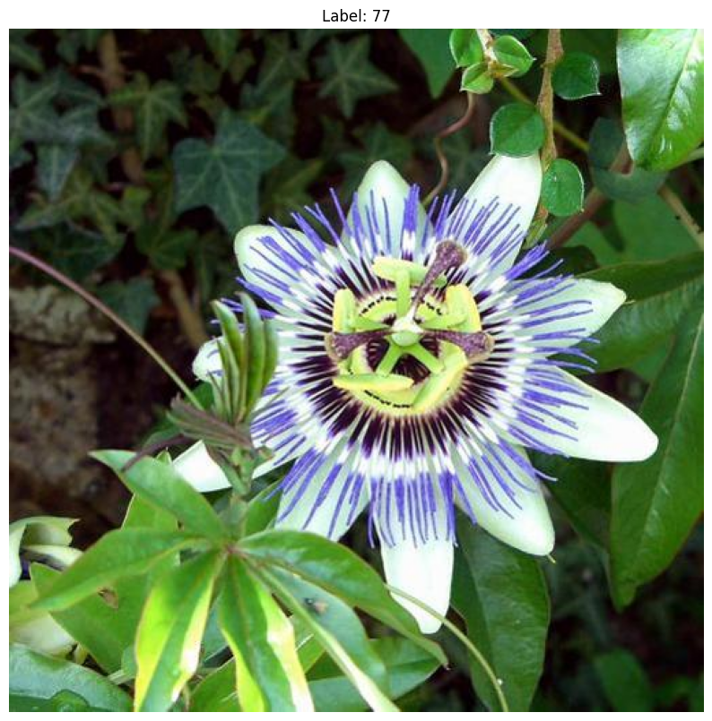
Plot some images from the dataset

for i in range(5):
    img, label, _ = train_dataset[i]
    print("Image size:", img.shape)
    plot_image(img, title=f"Label: {label}")

Image size: (500, 591, 3)

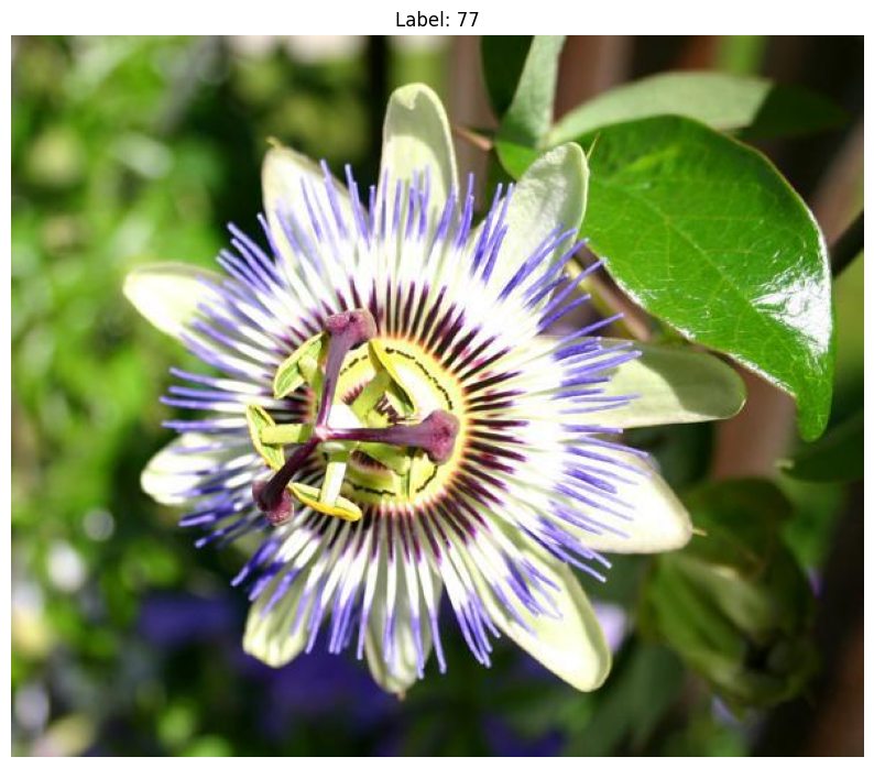
Image size: (500, 625, 3)

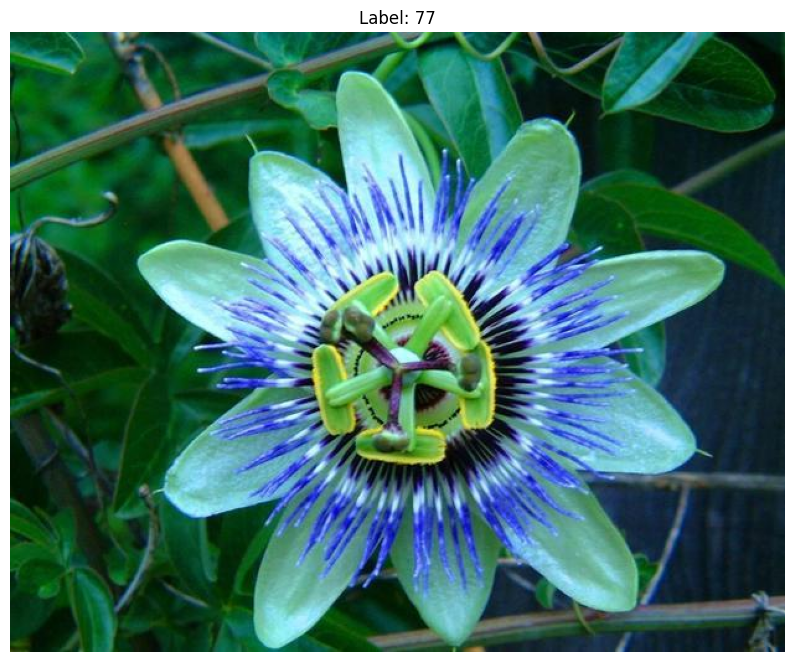
Image size: (667, 500, 3)

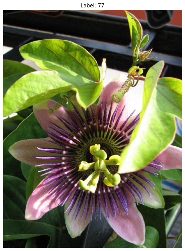
Image size: (500, 667, 3)

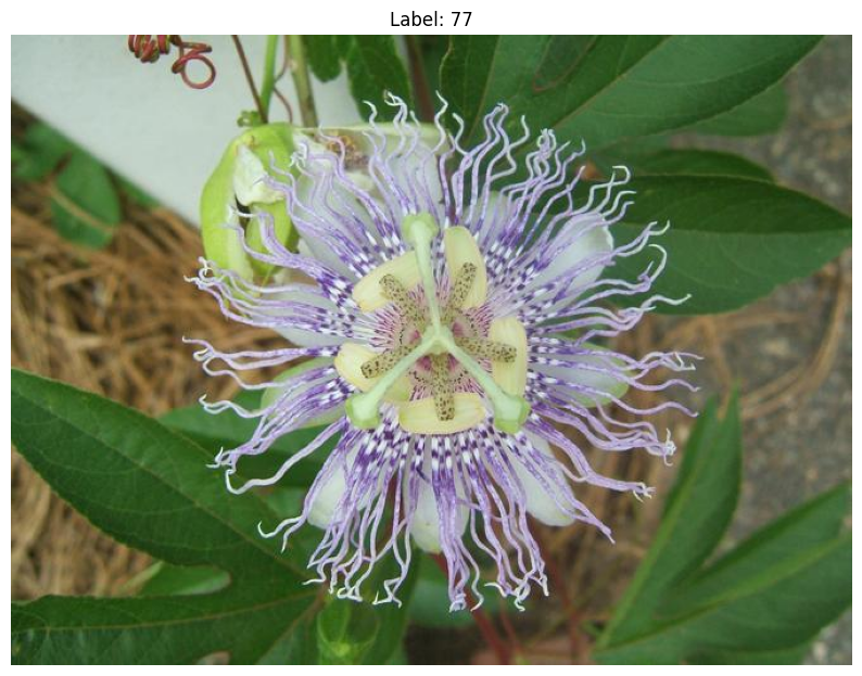
Image size: (500, 508, 3)

3. Extract deep convolutional features

In the original paper [1], SIFT and RootSIFT features were used. Hence, the default parameter of the embedding would be RootSIFT. However, here, I would like to demonstrate the usage of deep convolutional features, as mentioned in [2].

We use DeepConvFeature from our code. For demonstration, we’ll pick resnet18 and the last conv layer.

extractor = DeepConvFeature(
    backbone="resnet18",
    layer_index=-1,  # Last conv layer
)

Declare the VLAD embedder

vlad_embedder_no_pca = VLADEmbedder(feature_extractor=extractor, n_clusters=NUM_CLUSTERS)

The following cell trains the model from scratch on the training images. It might take quite a bit of time.

vlad_embedder_no_pca.learn(train_dataset[i][0] for i in train_indices)

/home/runner/work/Python-Visual-Similarity/Python-Visual-Similarity/.venv/lib/python3.10/site-packages/torchvision/transforms/functional.py:154: UserWarning: The given NumPy array is not writable, and PyTorch does not support non-writable tensors. This means writing to this tensor will result in undefined behavior. You may want to copy the array to protect its data or make it writable before converting it to a tensor. This type of warning will be suppressed for the rest of this program. (Triggered internally at /__w/pytorch/pytorch/torch/csrc/utils/tensor_numpy.cpp:213.)
  img = torch.from_numpy(pic.transpose((2, 0, 1))).contiguous()

[INFO] Learning the visual vocabulary with the following parameters:
   - Number of clusters: 32
   - Feature Extractor used: DeepConvFeature
   - Dimension of the feature space: 512

If you have issue with the runtime, you can follow this procedure instead:

1. Train the embedder once.

2. Save it using save_to_disk.

3. Load it back later using VLADEmbedder.load_from_disk.

Build the image store

This embeds the selected training images and indexes the embeddings in an InMemoryImageEmbeddingStore. The store will come handy as we do image retrieval later on. For that, we first need to compute some variables from the dataset.

paths = [train_dataset.image_paths[i] for i in train_indices]
labels_by_path = dict(zip(train_dataset.image_paths, train_dataset.labels, strict=True))

vlad_store = InMemoryImageEmbeddingStore(
    image_paths=paths, embedder=vlad_embedder_no_pca
)
vlad_store.build_store()

Similar to above, but here, the dimension of each feature vector is reduced by half using PCA.

Declare the VLAD embedder (with PCA)

vlad_embedder_with_pca = VLADEmbedder(feature_extractor=extractor, n_clusters=NUM_CLUSTERS)

vlad_embedder_with_pca.learn(
    (train_dataset[i][0] for i in train_indices), dim_reduction_factor=DIM_REDUCTION_FACTOR
)

[INFO] Learning the visual vocabulary with the following parameters:
   - Number of clusters: 32
   - Feature Extractor used: DeepConvFeature
   - Dimension of the feature space: 512

   - New dimension after PCA reduction: 256

vlad_store_pca = InMemoryImageEmbeddingStore(
    image_paths=paths, embedder=vlad_embedder_with_pca
)
vlad_store_pca.build_store()

5. Compare some images

We will now use the trained VLAD embedders to compute similarity between some images.

image_1, label_1, path_1 = train_dataset[2005]
image_2, label_2, path_2 = val_dataset[401]
plot_image(image_1)
plot_image(image_2)

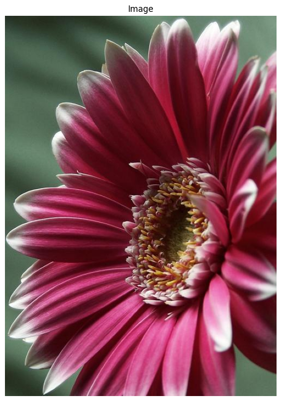
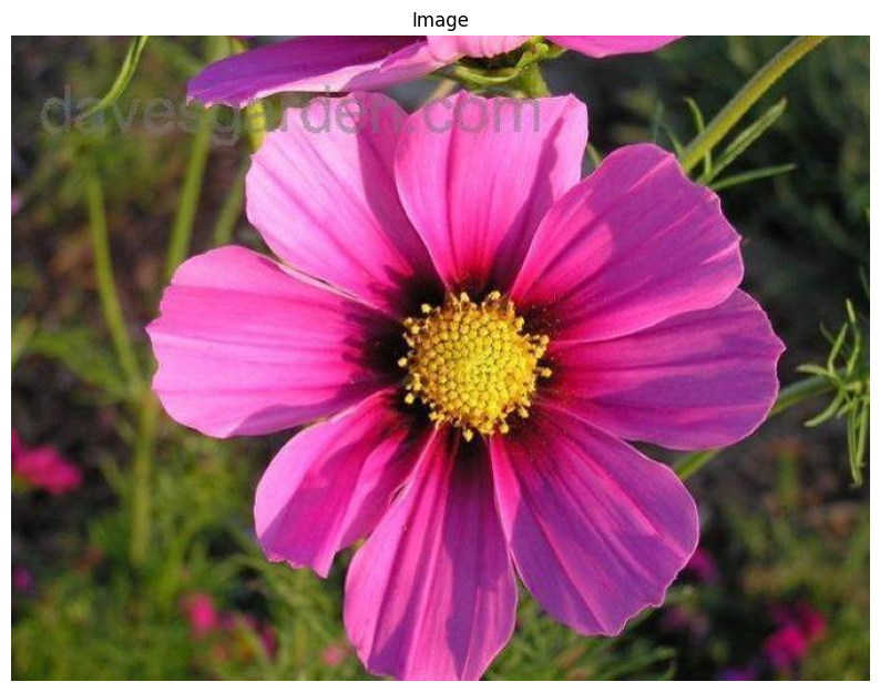
Now, we compare the two images. cosine similarity is used in this case.

sim_with_pca = vlad_embedder_with_pca.similarity_score(image_1, image_2)
print("Similarity Score, with PCA: ", sim_with_pca)
sim_without_pca = vlad_embedder_no_pca.similarity_score(image_1, image_2)
print("Similarity Score, without PCA: ", sim_without_pca)

Similarity Score, with PCA:  [[0.09383307]]
Similarity Score, without PCA:  [[0.11210608]]

6. Fetch the most similar image in the dataset, given a query image

Now, we will select an image in the validation dataset, on which the model is not yet trained:

query_image, query_label, query_path = val_dataset[103]

plot_image(query_image, title=f"Query image. Label: {query_label}")

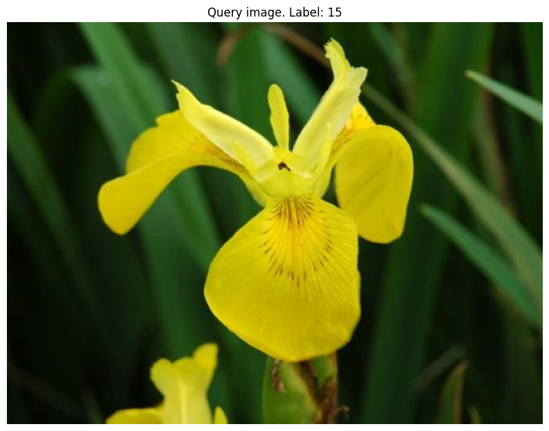
Retrieve top-k most similar images using the stores built above. We will see how it works, with and without PCA.

Each result is a Candidate holding the path of the retrieved image and its score. The stores are built in the cosine space, so the score is the cosine distance 1 - cosine_similarity, and lower means more similar.

top_k_vlad_pca = vlad_store_pca.retrieve_top_k_similar(query_image)[0]
print("Evaluation of VLAD with PCA:")
for candidate in top_k_vlad_pca:
    print(
        f"Path: {os.path.basename(candidate.path)}, Cosine distance: {candidate.score:.4f}"
    )

top_k_vlad_no_pca = vlad_store.retrieve_top_k_similar(query_image)[0]
print("\nEvaluation of VLAD without PCA:")
for candidate in top_k_vlad_no_pca:
    print(
        f"Path: {os.path.basename(candidate.path)}, Cosine distance: {candidate.score:.4f}"
    )

Evaluation of VLAD with PCA:
Path: image_04666.jpg, Cosine distance: 0.7206
Path: image_04684.jpg, Cosine distance: 0.7782
Path: image_00971.jpg, Cosine distance: 0.7845
Path: image_06389.jpg, Cosine distance: 0.7928
Path: image_01091.jpg, Cosine distance: 0.7944

Evaluation of VLAD without PCA:
Path: image_04666.jpg, Cosine distance: 0.7672
Path: image_01095.jpg, Cosine distance: 0.7948
Path: image_06389.jpg, Cosine distance: 0.7988
Path: image_06351.jpg, Cosine distance: 0.8005
Path: image_00971.jpg, Cosine distance: 0.8024

Let’s plot the top-k images next to each other.

a) Using Model trained on data with PCA

plot_candidates(query_image, query_label, top_k_vlad_pca, labels_by_path)

b) Using model trained on full data

plot_candidates(query_image, query_label, top_k_vlad_no_pca, labels_by_path)

7. Similar to above, we will do the exact things for the Fisher Vector

The implementation for both VLAD and Fisher Vectors are identical. After all, VLAD is simply a simplified case of Fisher Vector.

The Fisher Vectors are about twice as large as the VLAD vectors, so we free the memory held by the VLAD stores before building the Fisher Vector stores.

del vlad_store, vlad_store_pca

Instantiate Fisher Vector Embedder

fisher_embedder_no_pca = FisherVectorEmbedder(
    feature_extractor=extractor, n_components=NUM_CLUSTERS
)

The following cell trains the model from scratch as well. It might take quite a bit of time (even longer than VLAD).

fisher_embedder_no_pca.learn(train_dataset[i][0] for i in train_indices)

[INFO] Learning the visual vocabulary with the following parameters:
   - Number of clusters: 32
   - Feature Extractor used: DeepConvFeature
   - Dimension of the feature space: 512

Build the image store

fisher_store = InMemoryImageEmbeddingStore(
    image_paths=paths, embedder=fisher_embedder_no_pca
)
fisher_store.build_store()

Similar to above, if you run into runtime issues, consider saving the trained embedder using save_to_disk and loading it back later. You can also fit a Gaussian Mixture model in advance and pass it to load_clustering_model_from_sklearn. The Gaussian Mixture object can be imported as:

from sklearn.mixture import GaussianMixture

Note that only covariance_type="diag" is supported. Otherwise, the implementation is identical to that of VLADEmbedder.

Instantiate Fisher Vector Embedder with PCA

fisher_embedder_with_pca = FisherVectorEmbedder(
    feature_extractor=extractor, n_components=NUM_CLUSTERS
)

fisher_embedder_with_pca.learn(
    (train_dataset[i][0] for i in train_indices), dim_reduction_factor=DIM_REDUCTION_FACTOR
)

[INFO] Learning the visual vocabulary with the following parameters:
   - Number of clusters: 32
   - Feature Extractor used: DeepConvFeature
   - Dimension of the feature space: 512

   - New dimension after PCA reduction: 256

/home/runner/work/Python-Visual-Similarity/Python-Visual-Similarity/pyvisim/classic/_base_embedder.py:436: FutureWarning: Best of 1 EM run(s) did not converge within 100 iterations; consider raising max_iter, raising tol or increasing n_init.
  self._clustering_model.fit(features)

fisher_store_pca = InMemoryImageEmbeddingStore(
    image_paths=paths, embedder=fisher_embedder_with_pca
)
fisher_store_pca.build_store()

Compute similarity of two images

image_similarity_with_pca = fisher_embedder_with_pca.similarity_score(image_1, image_2)
image_similarity_without_pca = fisher_embedder_no_pca.similarity_score(image_1, image_2)
print("Fisher Similarity Score, with PCA: ", image_similarity_with_pca)
print("Fisher Similarity Score, without PCA: ", image_similarity_without_pca)

Fisher Similarity Score, with PCA:  [[0.03832705]]
Fisher Similarity Score, without PCA:  [[0.03631138]]

Retrieve top-k most similar images

plot_image(query_image, title=f"Query image. Label: {query_label}")

top_k_fisher_pca = fisher_store_pca.retrieve_top_k_similar(query_image)[0]
print("Evaluation of Fisher Vector with PCA:")
for candidate in top_k_fisher_pca:
    print(
        f"Path: {os.path.basename(candidate.path)}, Cosine distance: {candidate.score:.4f}"
    )

top_k_fisher_no_pca = fisher_store.retrieve_top_k_similar(query_image)[0]
print("\nEvaluation of Fisher Vector without PCA:")
for candidate in top_k_fisher_no_pca:
    print(
        f"Path: {os.path.basename(candidate.path)}, Cosine distance: {candidate.score:.4f}"
    )

Evaluation of Fisher Vector with PCA:
Path: image_06369.jpg, Cosine distance: 0.8665
Path: image_06351.jpg, Cosine distance: 0.8926
Path: image_06389.jpg, Cosine distance: 0.9013
Path: image_04655.jpg, Cosine distance: 0.9039
Path: image_00971.jpg, Cosine distance: 0.9054

Evaluation of Fisher Vector without PCA:
Path: image_04666.jpg, Cosine distance: 0.8373
Path: image_01095.jpg, Cosine distance: 0.8462
Path: image_01091.jpg, Cosine distance: 0.8539
Path: image_06389.jpg, Cosine distance: 0.8541
Path: image_04655.jpg, Cosine distance: 0.8606

Let’s plot top-k images next to each other.

a) Using Model trained on Data with PCA

plot_candidates(query_image, query_label, top_k_fisher_pca, labels_by_path)

b) Using Model trained on full data

plot_candidates(query_image, query_label, top_k_fisher_no_pca, labels_by_path)