4.1 Image Search

This notebook builds a searchable image gallery and queries it with an image rather than with text. The gallery is the Oxford 102 Flowers dataset [1], each image is turned into a feature vector by a pre-trained CLIP model [2], and the vectors are indexed in an HNSW graph [3] so that the nearest neighbors of a query are found without scanning the gallery.

The pipeline has four steps:

1. Embed: every gallery image is read and passed through ClipEmbedder, which returns one vector per image.

2. Index: the vectors are handed to the search index that InMemoryImageEmbeddingStore owns from then on.

3. Serialization: the store is written to a single safetensors file, embedder included, so the gallery never has to be embedded twice.

4. Query: an unseen image is embedded with the same embedder and matched against the index.

Note

Note that embedding the whole gallery takes a while. Once the file is on disk, the notebook can be restarted from the loading cell.

Hnsw Search Index

A brute-force search compares the query against every gallery vector, which is exact but linear in the size of the gallery. HNSW instead builds a multi-layer proximity graph over the vectors and walks it greedily, which reaches the neighborhood of the query in far fewer comparisons. The trade is recall: the answer is approximate, and how approximate is controlled by the parameters set below.

Further reading: Image Store and FAISS Indexes.

Import libraries

import matplotlib.pyplot as plt
import numpy as np
from PIL import Image

from pyvisim.datasets import OxfordFlowerDataset
from pyvisim.neural_networks import ClipEmbedder
from pyvisim.retrieval.image_store import InMemoryImageEmbeddingStore

/home/runner/work/Python-Visual-Similarity/Python-Visual-Similarity/.venv/lib/python3.10/site-packages/tqdm/auto.py:21: TqdmWarning: IProgress not found. Please update jupyter and ipywidgets. See https://ipywidgets.readthedocs.io/en/stable/user_install.html
  from .autonotebook import tqdm as notebook_tqdm

Hyperparameters

Note

IMAGE_STEP keeps every IMAGE_STEP-th image of the training split in the gallery. Set to 1 if you want to use all images.

IMAGE_STEP = 4

Build the image store

Constructing InMemoryImageEmbeddingStore only records the gallery. build_store() reads every path in image_paths, embeds it with embedder and hands the resulting matrix to the search index, so call it right after the constructor. Until then the store holds nothing, and searching it raises RuntimeError. Pass lazy_build=False to have the constructor call build_store() itself.

The gallery is every IMAGE_STEP-th image of the training split of Oxford 102 Flowers [1], which holds 6149 images.

Arguments:

• embedder: any object exposing an embed method. ClipEmbedder is used here, but the VLAD, Fisher Vector, Siamese and Triplet embedders fit here just as well.

• search_index: "hnsw" builds the graph, None falls back to an exact brute-force scan. A FAISS index [5] can be passed instead.

• index_params: forwarded to the index constructor. graph_degree is the number of bidirectional links created per node of the graph, build_candidates the size of the candidate list kept while building it. Both raise recall, graph_degree at the cost of memory and build_candidates at the cost of build time.

The metric space defaults to "cosine", which stores the vectors L2-normalised and scores them by 1 - cosine_similarity.

train_dataset = OxfordFlowerDataset()
train_indices = range(0, len(train_dataset), IMAGE_STEP)
train_image_paths = [train_dataset.image_paths[i] for i in train_indices]
print("Number of images in the gallery:", len(train_image_paths))

embedder = ClipEmbedder()

image_store = InMemoryImageEmbeddingStore(
    image_paths=train_image_paths,
    embedder=embedder,
    search_index="hnsw",
    index_params={"graph_degree": 16, "build_candidates": 200},
)
image_store.build_store()
image_store.save_to_disk("flower_image_store.safetensors")

Number of images in the gallery: 1538

Warning: You are sending unauthenticated requests to the HF Hub. Please set a HF_TOKEN to enable higher rate limits and faster downloads.

PosixPath('flower_image_store.safetensors')

Load the store back from disk

The saved file carries the embedder as well, so the store is rebuilt without touching the original images and without downloading the CLIP weights again. The index is rebuilt from the saved embeddings, using the parameters it was saved with.

This is the entry point for a fresh session. Run the import cell, then this one, and skip the embedding cell above entirely. A store loaded from disk is already built, so it needs no build_store() call.

One caveat applies to FAISS indexes only. A FAISS index cannot be written into the file, so a rebuilt one has to be handed back as search_index=.... Without it the store falls back to an exact brute-force scan over the saved embeddings and warns about the fallback.

image_store = InMemoryImageEmbeddingStore.load_from_disk(
    "flower_image_store.safetensors"
)

Helper to display images>

def _gallery_labels_by_path():
    dataset = OxfordFlowerDataset()
    return dict(zip(dataset.image_paths, dataset.labels, strict=True))


#: Class id of every gallery image, keyed by its path.
GALLERY_LABELS_BY_PATH = _gallery_labels_by_path()


def _as_rgb_array(image_array_or_path):
    if isinstance(image_array_or_path, np.ndarray):
        return image_array_or_path
    with Image.open(image_array_or_path) as image:
        return np.asarray(image.convert("RGB"))


def visualize_image(image_array_or_path, title=None):
    plt.figure(figsize=(4, 4))
    plt.imshow(_as_rgb_array(image_array_or_path))
    plt.axis("off")
    if title is not None:
        plt.title(title)
    plt.show()


def visualize_candidate(candidate):
    label = GALLERY_LABELS_BY_PATH[candidate.path]
    visualize_image(
        candidate.path, title=f"label {label}, score = {candidate.score:.4f}"
    )

The query image

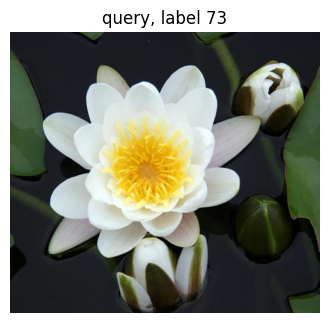
The query is drawn from the test split, so it was never embedded into the gallery and the search has to generalise to an unseen image. Its own class label is shown above it, and it is the label every retrieved image is measured against further down.

test_dataset = OxfordFlowerDataset(purpose="test")
image1, label1, _ = test_dataset[172]
visualize_image(image1, title=f"query, label {label1}")

Retrieve the nearest neighbors

retrieve_top_k_similar embeds the query with the store’s own embedder, walks the index, and maps the returned row ids back to gallery paths.

It takes a batch as readily as a single image and always returns one ranked list per query, which is why the first list is unpacked with [0]. Batching is worth using whenever there is more than one query, because the index answers a single (M, D) matrix far faster than it answers M separate queries.

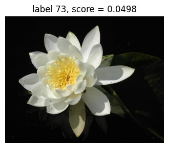
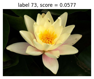
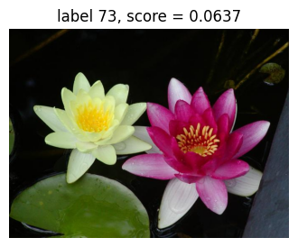
Each result is a Candidate, a named tuple of path and score, ordered best first. In cosine space the score is 1 - cosine_similarity, so lower means more similar and a near-duplicate of the query scores close to 0.0.

Query time is bounded by search_candidates, the width of the graph walk, which defaults to 50. Asking for more than search_candidates neighbors raises it to k automatically.

candidates = image_store.retrieve_top_k_similar(image1, k=5)[0]

Inspect the results

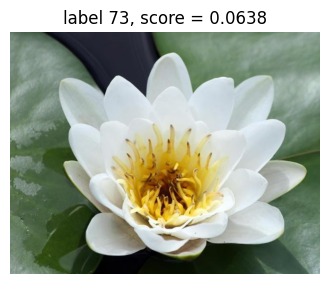
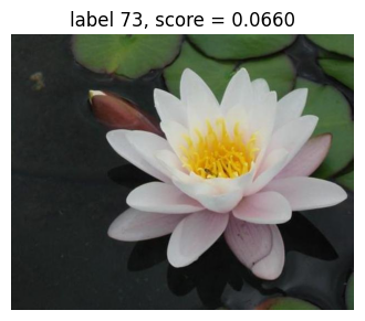
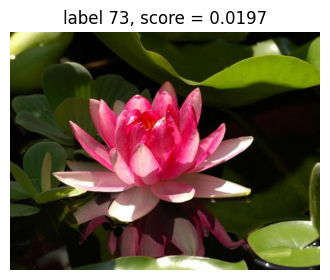
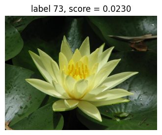
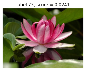
The top matches should carry the query’s own class label. HNSW is approximate, so a graph built for speed can miss a true neighbor. If the results look poor, rebuild with a larger graph_degree or build_candidates, or raise search_candidates at query time. Building the store with search_index=None gives the exact ranking to compare against, at the cost of scanning the whole gallery on every query.

for candidate in candidates:
    visualize_candidate(candidate)

Refine the query with alpha query expansion

A query is a single point, and a single point can sit off to the side of the group it belongs to. Alpha query expansion (aQE) [7] moves it back towards the middle of that group before the ranking is decided.

The store searches once, reads the embeddings of the expansion_neighbors best matches back off the index, and replaces the query by the L2-normalised weighted average of itself and those matches. Each match is weighted by its cosine similarity to the query raised to expansion_alpha, so a close match pulls harder than a distant one, and a match whose similarity is not positive does not pull at all. The final search then runs with the refined query.

Arguments:

• query_expansion: turns the refinement on. It is off by default, because it costs one extra index search per query plus the decoding of expansion_neighbors gallery vectors.

• expansion_alpha: exponent of the similarity weights. 0 weights every match with a positive similarity alike, which is the classic average query expansion.

• expansion_neighbors: how many of the top-ranked gallery images are averaged into the query.

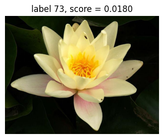
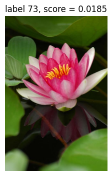
The scores below are still the store’s own distances, so lower still means more similar, but they are measured from the refined query rather than from the one that was embedded and are not comparable to the scores above.

expanded_candidates = image_store.retrieve_top_k_similar(
    image1,
    k=5,
    query_expansion=True,
    expansion_alpha=3.0,
    expansion_neighbors=50,
)[0]

for expanded_candidate in expanded_candidates:
    visualize_candidate(expanded_candidate)

Re-rank the candidates with k-reciprocal encoding

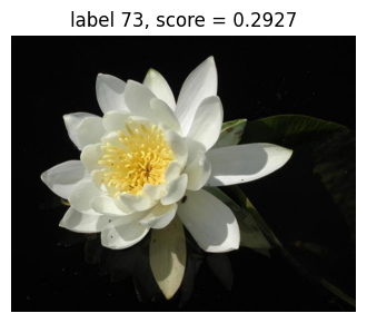
Query expansion changes the query. Re-ranking leaves the query untouched and re-orders a pool of candidates that has already been retrieved.

KReciprocalReranker [8] asks of every candidate whether the query lies among its own nearest neighbors, not only whether it lies among the query’s. That relation is far stricter than plain proximity: a false match can sit close to the query while the query sits nowhere near the false match’s own neighbors. The query and every candidate are encoded into a k-reciprocal feature, a vector that holds a weight for each of their k-reciprocal neighbors and zero elsewhere, and the Jaccard distance between two such features says how much the two neighborhoods agree.

The neighborhoods are built among the candidates themselves, so a pool no larger than the answer leaves them nothing to say. A pool of 100 is retrieved below and the best five are kept.

Arguments:

• k1: size of the neighborhoods the k-reciprocal sets are built from. The pool should hold at least this many candidates.

• k2: size of the neighborhood the local query expansion averages the features over. 1 turns that step off.

• lambda_value: weight of the original distance in the final one, from 0 (Jaccard distance only) to 1 (original ranking kept).

• top_k: how many of the re-ranked candidates rerank returns.

The scores are the final distances of the re-ranking rather than the store’s. They lie in [0, 1], and lower again means more similar.

Further reading: Re-ranking.

from pyvisim.retrieval.reranking import KReciprocalReranker

reranker = KReciprocalReranker(image_store, k1=20, k2=6, lambda_value=0.3)

candidate_pool = image_store.retrieve_top_k_similar(image1, k=100)[0]
reranked_candidates = reranker.rerank(candidate_pool, top_k=5)

for reranked_candidate in reranked_candidates:
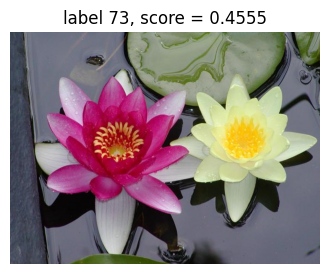
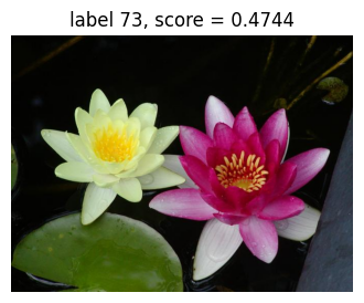
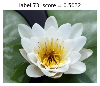
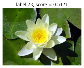
    visualize_candidate(reranked_candidate)

Search through a FAISS index

The store can also search through a FAISS index, so an algorithm this package does not ship can still be used over the same gallery. The example below rebuilds the HNSW graph with FAISS [5] and hands it over.

The graph is built over image_store.embeddings, the matrix the store’s own index holds, so the gallery is never embedded a second time.

Two things are the caller’s job here rather than the store’s:

• The metric. METRIC_INNER_PRODUCT ranks by cosine similarity only if the vectors are L2-normalised. They already are, because the store was built in the default "cosine" space, and the queries arrive normalised too, because ClipEmbedder normalises what it returns.

• The parameters. index_params only configures the built-in indexes, so the store rejects it for a FAISS index. m is a constructor argument of IndexHNSWFlat, while efConstruction and efSearch are set on the graph itself.

A FAISS index already holds the gallery, so a store on one is built as soon as it is constructed and needs no build_store() call.

The store reads the gallery vectors back off the index, which IndexHNSWFlat can do because it keeps them uncompressed.

import faiss

gallery_vectors = image_store.embeddings

faiss_index = faiss.IndexHNSWFlat(
    gallery_vectors.shape[1], 16, faiss.METRIC_INNER_PRODUCT
)
faiss_index.hnsw.efConstruction = 200
faiss_index.add(gallery_vectors)
faiss_index.hnsw.efSearch = 50

faiss_store = InMemoryImageEmbeddingStore(
    image_paths=image_store.paths,
    embedder=embedder,
    search_index=faiss_index,
)
faiss_store

InMemoryImageEmbeddingStore(num_images=1538, dim=512, index_name='faiss.IndexHNSWFlat', space='ip')

Compare the two rankings

Both stores report distances, so lower means more similar in both columns. The FAISS index was built for inner products, so the store searches it in the "ip" space and scores a match by 1 - inner_product. The built-in index returns the 1 - cosine_similarity distance of its "cosine" space. On L2-normalised vectors the two are the same quantity, so both columns can be read against each other directly.

Both graphs are approximate and are built by different code, so the two rankings are free to disagree on a borderline neighbor. On this query they do not.

faiss_candidates = faiss_store.retrieve_top_k_similar(image1, k=5)[0]

for faiss_candidate, hnsw_candidate in zip(faiss_candidates, candidates, strict=True):
    agreement = "same" if faiss_candidate.path == hnsw_candidate.path else "differs"
    print(
        f"{agreement:>7}  faiss={faiss_candidate.score:.4f}  "
        f"hnsw={hnsw_candidate.score:.4f}  {faiss_candidate.path}"
    )

   same  faiss=0.0498  hnsw=0.0498  /home/runner/.cache/pyvisim/oxford_flower_dataset/images/jpg/image_00345.jpg
   same  faiss=0.0577  hnsw=0.0577  /home/runner/.cache/pyvisim/oxford_flower_dataset/images/jpg/image_00371.jpg
   same  faiss=0.0637  hnsw=0.0637  /home/runner/.cache/pyvisim/oxford_flower_dataset/images/jpg/image_00435.jpg
   same  faiss=0.0638  hnsw=0.0638  /home/runner/.cache/pyvisim/oxford_flower_dataset/images/jpg/image_00299.jpg
   same  faiss=0.0660  hnsw=0.0660  /home/runner/.cache/pyvisim/oxford_flower_dataset/images/jpg/image_00316.jpg

Serialize a store built on a FAISS index

save_to_disk writes the embeddings, the paths and the embedder, but not the FAISS index itself, which this library cannot serialize. Loading therefore takes the index back as search_index=..., and its type is checked against the saved one, faiss.IndexHNSWFlat here, so a mismatch is reported. Left out, the store falls back to an exact brute-force scan over the saved embeddings and warns about it.

A quantized index needs embeddings=... passed to save_to_disk as well, because what it reconstructs is an approximation of the embeddings rather than the embeddings themselves.

Note that the file written below is a second full copy of the gallery, roughly the size of the one written further up.

faiss_store.save_to_disk("flower_faiss_store.safetensors")

restored_store = InMemoryImageEmbeddingStore.load_from_disk(
    "flower_faiss_store.safetensors",
    search_index=faiss_index,
)
restored_candidates = restored_store.retrieve_top_k_similar(image1, k=5)[0]

for restored_candidate in restored_candidates:
    print(f"{restored_candidate.score:.4f}  {restored_candidate.path}")

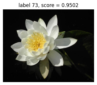
0.0498  /home/runner/.cache/pyvisim/oxford_flower_dataset/images/jpg/image_00345.jpg
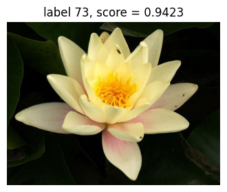
0.0577  /home/runner/.cache/pyvisim/oxford_flower_dataset/images/jpg/image_00371.jpg
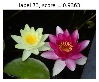
0.0637  /home/runner/.cache/pyvisim/oxford_flower_dataset/images/jpg/image_00435.jpg
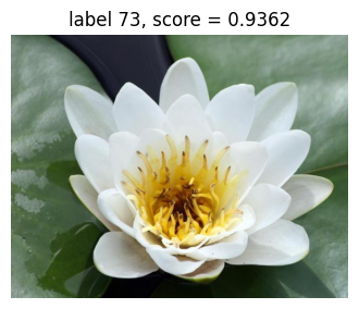
0.0638  /home/runner/.cache/pyvisim/oxford_flower_dataset/images/jpg/image_00299.jpg
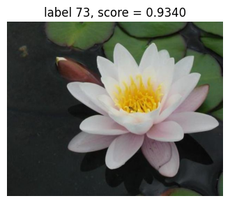
0.0660  /home/runner/.cache/pyvisim/oxford_flower_dataset/images/jpg/image_00316.jpg

Visualise the results

It can be observed that the results are identical to the ones returned by the built-in index, since the same hnsw parameters are used.

The scores in the titles are the 1 - inner_product distances of the store, so here too lower means more similar. The labels are read the same way as everywhere else.

Now, you can plug in any FAISS index you like for the search.

for faiss_candidate in faiss_candidates:
    visualize_candidate(faiss_candidate)

References

[1] Nilsback, M.-E., & Zisserman, A. (2008). Automated Flower Classification over a Large Number of Classes. In Proceedings of the Sixth Indian Conference on Computer Vision, Graphics and Image Processing (ICVGIP), 722-729. https://www.robots.ox.ac.uk/~vgg/data/flowers/102/

[2] Radford, A., Kim, J. W., Hallacy, C., Ramesh, A., Goh, G., Agarwal, S., Sastry, G., Askell, A., Mishkin, P., Clark, J., Krueger, G., & Sutskever, I. (2021). Learning Transferable Visual Models From Natural Language Supervision. In Proceedings of the 38th International Conference on Machine Learning (ICML), PMLR 139, 8748-8763. https://arxiv.org/abs/2103.00020

[3] Malkov, Y. A., & Yashunin, D. A. (2020). Efficient and Robust Approximate Nearest Neighbor Search Using Hierarchical Navigable Small World Graphs. IEEE Transactions on Pattern Analysis and Machine Intelligence, 42(4), 824-836. https://arxiv.org/abs/1603.09320

[4] hnswlib, the reference implementation the compiled index is built on. https://github.com/nmslib/hnswlib

[5] Johnson, J., Douze, M., & Jegou, H. (2019). Billion-Scale Similarity Search with GPUs. IEEE Transactions on Big Data, 7(3), 535-547. https://arxiv.org/abs/1702.08734

[6] Pinecone. Hierarchical Navigable Small Worlds (HNSW). https://www.pinecone.io/learn/series/faiss/hnsw/

[7] Radenovic, F., Tolias, G., & Chum, O. (2019). Fine-tuning CNN Image Retrieval with No Human Annotation. IEEE Transactions on Pattern Analysis and Machine Intelligence, 41(7), 1655-1668. https://arxiv.org/abs/1711.02512

[8] Zhong, Z., Zheng, L., Cao, D., & Li, S. (2017). Re-ranking Person Re-identification with k-reciprocal Encoding. In Proceedings of the IEEE Conference on Computer Vision and Pattern Recognition (CVPR), 1318-1327. https://arxiv.org/abs/1701.08398