2.4 Custom Feature Extractor with RootSIFT

Note

Training the k-means model on every training image takes quite a bit of time. IMAGE_STEP keeps every IMAGE_STEP-th training image to train the embedder. Set it to 1 if you want to use all images.

This notebook demonstrates how to write your own feature extractor by inheriting from FeatureExtractorBase. For this, a RootSIFT implementation on top of the SIFT implementation of OpenCV is used s a feature extractor instead of the built-in RootSIFT module, offering significantly more speed, at the cost of an opencv installation. It is then used to train a VLADEmbedder on the Oxford Flowers dataset and to compare two images.

Import libraries

import cv2
import numpy as np
from matplotlib import pyplot as plt
import torch

from pyvisim.base import FeatureExtractorBase
from pyvisim.classic import VLADEmbedder
from pyvisim.datasets import OxfordFlowerDataset
from pyvisim.typing import Float32NumpyArray, MatLike
from pyvisim.utils.image_utils import to_single_image

Hyperparameters

NUM_CLUSTERS is the number of visual words of the VLAD vocabulary, DIM_REDUCTION_FACTOR reduces the dimension of the descriptors by half using PCA before the vocabulary is learned, and NUM_FEATURES is the maximum number of keypoints SIFT detects per image.

NUM_CLUSTERS = 32
DIM_REDUCTION_FACTOR = 2
IMAGE_STEP = 6
NUM_FEATURES = 500

Helper functions

def plot_image(image: np.ndarray | torch.Tensor, title: str = "Image") -> None:
    plt.figure(figsize=(10, 10))
    if isinstance(image, torch.Tensor):
        image = image.detach().cpu()
        if image.ndim == 3:
            image = image.permute(1, 2, 0)
        image = image.numpy()
    plt.imshow(image)
    plt.axis("off")
    plt.title(title)
    plt.show()

Declare the dataset

train_dataset = OxfordFlowerDataset(purpose="train")
val_dataset = OxfordFlowerDataset(purpose="validation")
print("Number of images in the dataset:", len(train_dataset))

train_indices = range(0, len(train_dataset), IMAGE_STEP)
print("Number of images used for training:", len(train_indices))

Number of images in the dataset: 6149
Number of images used for training: 1025

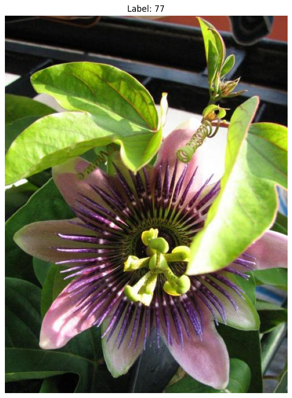
Plot some images from the dataset

for i in range(3):
    img, label, _ = train_dataset[i]
    print("Image size:", img.shape)
    plot_image(img, title=f"Label: {label}")

Image size: (500, 591, 3)

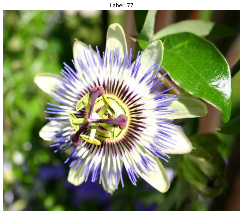
Image size: (500, 625, 3)

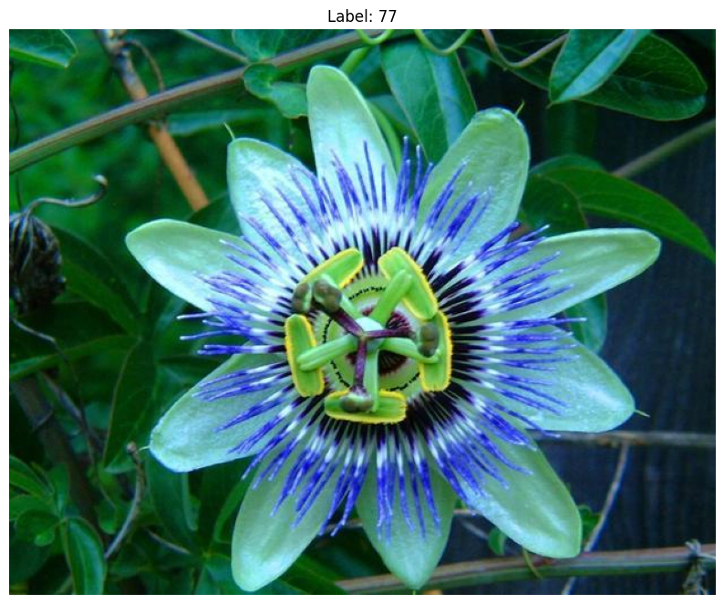
Image size: (667, 500, 3)

Write the RootSIFT feature extractor

A feature extractor maps one image to an (N, D) array of local descriptors, which an embedder then aggregates into a single vector. Following methods must be implemented:

• output_dim: the dimension D of one descriptor.

• __call__: takes one image and returns its descriptors as a float32 array of shape (N, output_dim).

__call__ accepts any MatLike image (a NumPy array, a torch tensor or an array-like object) in the layout given by dims and the value range given by value_range. to_single_image converts it into the canonical uint8 array of shape (H, W, C), or (H, W) for a grayscale input.

RootSIFT [2] starts from the SIFT [1] descriptors computed by OpenCV, 128 values per keypoint. Each descriptor is divided by its L1 norm, and then every value is replaced by its square root. Comparing two RootSIFT descriptors with the Euclidean distance is then the same as comparing the original SIFT descriptors with the Hellinger kernel, which suits histograms such as SIFT better [2].

class OpenCV_RootSIFT(FeatureExtractorBase):
    """
    Scale-Invariant Feature Transform with Hellinger kernel (RootSIFT) feature extractor.

    :param n_features: Maximum number of keypoints to detect per image.
    """

    def __init__(self, n_features: int = 500) -> None:
        super().__init__()
        self._sift = cv2.SIFT_create(nfeatures=n_features)

    @property
    def output_dim(self) -> int:
        return self._sift.descriptorSize()

    def __call__(
        self,
        image: MatLike,
        /,
        *,
        dims: str = "HWC",
        value_range: tuple[float, float] = (0.0, 255.0),
    ) -> Float32NumpyArray:
        canonical = to_single_image(image, dims=dims, value_range=value_range)
        grayscale = (
            cv2.cvtColor(canonical, cv2.COLOR_RGB2GRAY)
            if canonical.ndim == 3
            else canonical
        )
        _, descriptors = self._sift.detectAndCompute(grayscale, None)
        if descriptors is None:
            return np.zeros((0, self.output_dim), dtype=np.float32)
        descriptors = descriptors / (descriptors.sum(axis=1, keepdims=True) + 1e-7)
        return np.sqrt(descriptors)

Let’s check the extractor on one image. Every row of the output is the descriptor of one keypoint.

extractor = OpenCV_RootSIFT(n_features=NUM_FEATURES)
descriptors = extractor(train_dataset[0][0])
print("Output dimension:", extractor.output_dim)
print("Descriptors shape:", descriptors.shape)
print("Descriptors dtype:", descriptors.dtype)

Output dimension: 128
Descriptors shape: (501, 128)
Descriptors dtype: float32

Declare the VLAD embedder

The extractor is passed to the VLADEmbedder [3]. The embedder calls the extractor on every image, reduces the descriptors with PCA and clusters them into NUM_CLUSTERS visual words.

vlad_embedder = VLADEmbedder(feature_extractor=extractor, n_clusters=NUM_CLUSTERS)

The following cell trains the model from scratch on the training images. The dimension of the descriptors is reduced by half using PCA before the k-means model is trained. It might take quite a bit of time.

vlad_embedder.learn(
    (train_dataset[i][0] for i in train_indices), dim_reduction_factor=DIM_REDUCTION_FACTOR
)

[INFO] Learning the visual vocabulary with the following parameters:
   - Number of clusters: 32
   - Feature Extractor used: OpenCV_RootSIFT
   - Dimension of the feature space: 128

   - New dimension after PCA reduction: 64

Compare two images

Now, we pick a reference image, a similar image and a dissimilar image from the validation set, on which the model is not trained.

image_ref, label_ref, _ = val_dataset[2]
image_similar, label_similar, _ = val_dataset[3]
image_dissimilar, label_dissimilar, _ = val_dataset[100]
plot_image(image_ref, title=f"Reference Image. Label: {label_ref}")
plot_image(image_similar, title=f"Similar Image. Label: {label_similar}")
plot_image(image_dissimilar, title=f"Dissimilar Image. Label: {label_dissimilar}")

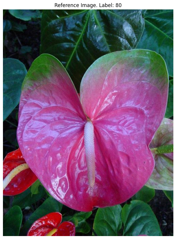
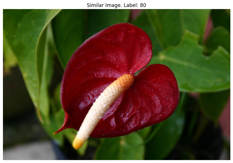
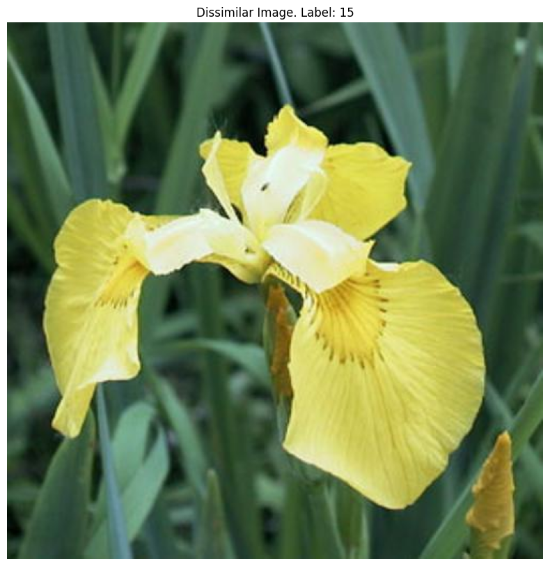
Now, we compare the reference image with the other two. cosine similarity is used in this case, so the score lies in [-1, 1] and a higher score means more similar.

score_similar = vlad_embedder.similarity_score(image_ref, image_similar).item()
print(f"Similarity score, similar pair: {score_similar:.4f}")

score_dissimilar = vlad_embedder.similarity_score(image_ref, image_dissimilar).item()
print(f"Similarity score, dissimilar pair: {score_dissimilar:.4f}")

Similarity score, similar pair: 0.1595
Similarity score, dissimilar pair: -0.0584

References

[1] Lowe, D. G. (2004). Distinctive image features from scale-invariant keypoints. International Journal of Computer Vision, 60(2), 91-110. https://doi.org/10.1023/B:VISI.0000029664.99615.94

[2] Arandjelović, R., & Zisserman, A. (2012). Three things everyone should know to improve object retrieval. In 2012 IEEE Conference on Computer Vision and Pattern Recognition (CVPR), 2911-2918. https://doi.org/10.1109/CVPR.2012.6248018

[3] Arandjelović, R., & Zisserman, A. (2013). All About VLAD. In 2013 IEEE Conference on Computer Vision and Pattern Recognition (CVPR), 1578-1585. https://doi.org/10.1109/CVPR.2013.207