2.1 Classical Embedding algorithms: VLAD and Fisher Vectors
Note
Extracting the descriptors and training the clustering models on every training image takes quite a bit of time. IMAGE_STEP keeps every IMAGE_STEP-th training image to train the embedders. Set it to 1 if you want to use all images.
Vector of Locally Aggregated Descriptors (VLAD) [3] and Fisher Vectors [4] turn the local descriptors of an image into a single vector of fixed size. Both first learn a visual vocabulary from the descriptors of the training images: VLAD clusters them with k-means, and the Fisher Vector fits a Gaussian mixture model to them.
This notebook trains both embedders on RootSIFT descriptors of the Oxford Flowers dataset in two ways:
With
learn, which extracts the descriptors, fits thePCAand fits the clustering model in one call. This uses this library’s built-in clustering and PCA implementations and hence spare ascikit-learninstallation.With
scikit-learnestimators: if you need extensive training capabilities ofscikit-learn, you can train your ownPCAand clustering models first, and then transfer their parameters to the embedders withload_clustering_model_from_sklearnandload_pca_model_from_sklearn.
Import libraries
import numpy as np
import torch
from matplotlib import pyplot as plt
from sklearn.cluster import KMeans
from sklearn.decomposition import PCA
from sklearn.mixture import GaussianMixture

from pyvisim.base import FeatureExtractorBase
from pyvisim.classic import FisherVectorEmbedder, VLADEmbedder
from pyvisim.datasets import OxfordFlowerDataset
from pyvisim.typing import Float32NumpyArray, MatLike
from pyvisim.utils.image_utils import to_single_image
Hyperparameters
NUM_CLUSTERS is the size of the visual vocabulary: the number of k-means clusters for VLAD and the number of Gaussian components for the Fisher Vector. DIM_REDUCTION_FACTOR halves the dimension of the descriptors with PCA before the vocabulary is learned, and SEED makes the training reproducible.
NUM_CLUSTERS = 32
DIM_REDUCTION_FACTOR = 2
IMAGE_STEP = 6
SEED = 0
Helper functions
def plot_image(image: np.ndarray | torch.Tensor, title: str = "Image") -> None:
    plt.figure(figsize=(10, 10))
    if isinstance(image, torch.Tensor):
        image = image.detach().cpu()
        if image.ndim == 3:
            image = image.permute(1, 2, 0)
        image = image.numpy()
    plt.imshow(image)
    plt.axis("off")
    plt.title(title)
    plt.show()


def print_similarity_scores(
    embedder: VLADEmbedder | FisherVectorEmbedder,
    reference: MatLike,
    similar: MatLike,
    dissimilar: MatLike,
) -> None:
    score_similar = embedder.similarity_score(reference, similar).item()
    score_dissimilar = embedder.similarity_score(reference, dissimilar).item()
    print(f"Similarity score, similar pair: {score_similar:.4f}")
    print(f"Similarity score, dissimilar pair: {score_dissimilar:.4f}")
Declare the dataset
train_dataset = OxfordFlowerDataset(purpose="train")
val_dataset = OxfordFlowerDataset(purpose="validation")
print("Number of images in the dataset:", len(train_dataset))

train_indices = range(0, len(train_dataset), IMAGE_STEP)
print("Number of images used for training:", len(train_indices))
Number of images in the dataset: 6149
Number of images used for training: 1025
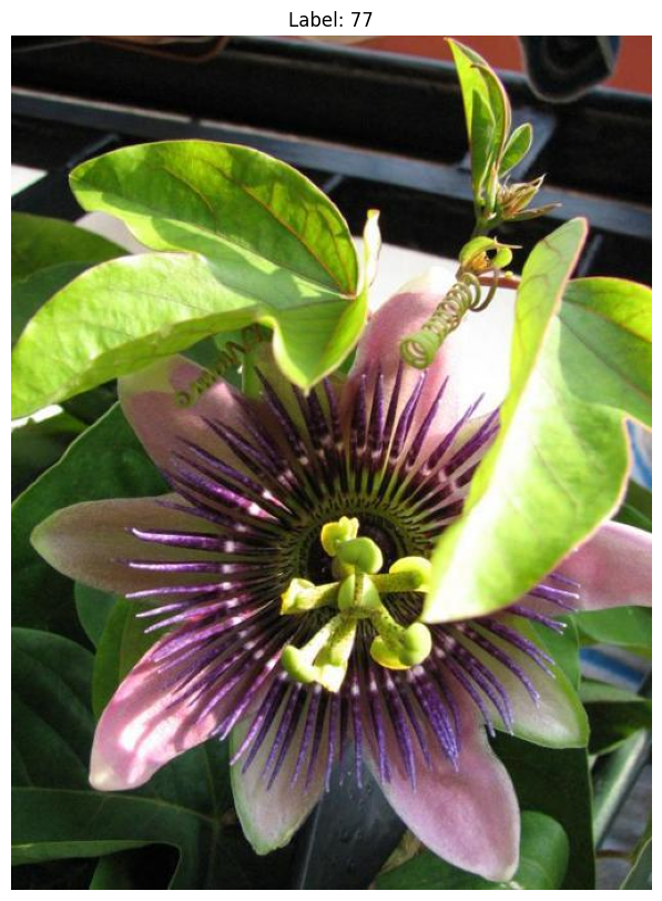
Plot some images from the dataset
for i in range(3):
    img, label, _ = train_dataset[i]
    print("Image size:", img.shape)
    plot_image(img, title=f"Label: {label}")
Image size: (500, 591, 3)
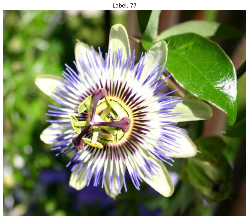
Image size: (500, 625, 3)
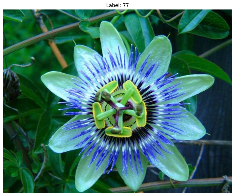
Image size: (667, 500, 3)
Declare the RootSIFT feature extractor
from pyvisim.features import RootSIFT
Note
The RootSIFT implementation of this library is written in Python, and hence not as performant as OpenCV's. If you need more speed, create your own feature extractor (see class OpenCV_RootSIFT below) using OpenCV. This is further covered in the RootSIFT tutorial.
from pyvisim.lazy_import import OptionalImport

with OptionalImport(err_msg = "OpenCV is not installed. Please install it with `pip install opencv-python-headless`") as cv2_import:
    import cv2


class OpenCV_RootSIFT(FeatureExtractorBase):
    """
    Scale-Invariant Feature Transform with Hellinger kernel (RootSIFT) feature extractor.
    """

    def __init__(self) -> None:
        super().__init__()
        cv2_import.check()
        self._sift = cv2.SIFT_create()

    @property
    def output_dim(self) -> int:
        return self._sift.descriptorSize()

    def __call__(
        self,
        image: MatLike,
        /,
        *,
        dims: str = "HWC",
        value_range: tuple[float, float] = (0.0, 255.0),
    ) -> Float32NumpyArray:
        canonical = to_single_image(image, dims=dims, value_range=value_range)
        grayscale = (
            cv2.cvtColor(canonical, cv2.COLOR_RGB2GRAY)
            if canonical.ndim == 3
            else canonical
        )
        _, descriptors = self._sift.detectAndCompute(grayscale, None)
        if descriptors is None:
            return np.zeros((0, self.output_dim), dtype=np.float32)
        descriptors = descriptors / (descriptors.sum(axis=1, keepdims=True) + 1e-7)
        return np.sqrt(descriptors)
# To speed up CI on GitHub Actions, OpenCV_RootSIFT is used instead of the built-in RootSIFT implementation. Comment in
# the line below to use the built-in RootSIFT, which saves the dependency on OpenCV, but is slower.
# extractor = RootSIFT()

extractor = OpenCV_RootSIFT()
Pick the images to compare
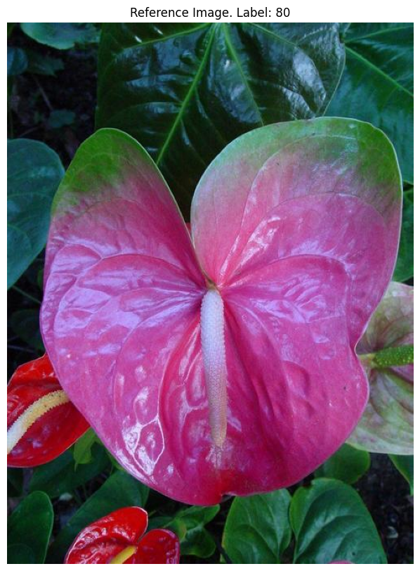
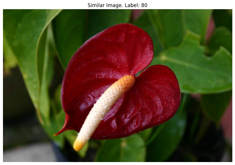
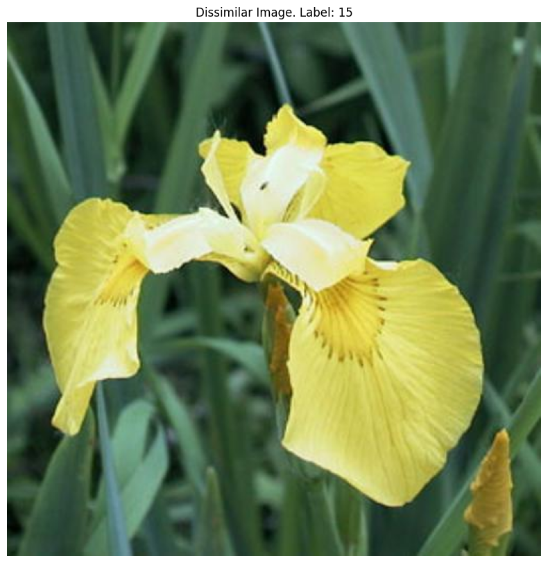
Every trained embedder scores the same three images from the validation set, on which none of them is trained: a reference image, a similar image of the same class and a dissimilar image of another class.
image_ref, label_ref, _ = val_dataset[2]
image_similar, label_similar, _ = val_dataset[3]
image_dissimilar, label_dissimilar, _ = val_dataset[100]
plot_image(image_ref, title=f"Reference Image. Label: {label_ref}")
plot_image(image_similar, title=f"Similar Image. Label: {label_similar}")
plot_image(image_dissimilar, title=f"Dissimilar Image. Label: {label_dissimilar}")
VLAD
VLAD assigns every descriptor of an image to its nearest k-means centroid and sums the residuals, the differences between the descriptors and their centroid, per cluster. The sums of all clusters are concatenated into one vector of size K * D, where K equals NUM_CLUSTERS and D is the dimension of the descriptors after PCA.
Train with learn
learn extracts the descriptors of the training images, fits a PCA that keeps output_dim // DIM_REDUCTION_FACTOR components and fits the k-means model on the projected descriptors. The options of the k-means model go into kmeans_params. The following cell might take quite a bit of time.
vlad_embedder = VLADEmbedder(
    feature_extractor=extractor, n_clusters=NUM_CLUSTERS, kmeans_params={"rng": SEED}
)
vlad_embedder.learn(
    (train_dataset[i][0] for i in train_indices), dim_reduction_factor=DIM_REDUCTION_FACTOR
)
[INFO] Learning the visual vocabulary with the following parameters:
   - Number of clusters: 32
   - Feature Extractor used: OpenCV_RootSIFT
   - Dimension of the feature space: 128
- New dimension after PCA reduction: 64
Train with scikit-learn
To use scikit-learn, you extract the descriptors yourself. The extractor returns one (N, D) array per image, and np.vstack stacks them into a single matrix.
descriptors = np.vstack([extractor(train_dataset[i][0]) for i in train_indices])
print("Descriptors shape:", descriptors.shape)
Descriptors shape: (1276476, 128)
Next comes the PCA.
pca = PCA(
    n_components=extractor.output_dim // DIM_REDUCTION_FACTOR,
    whiten=True,
    svd_solver="randomized",
    random_state=SEED,
)
projected_descriptors = pca.fit_transform(descriptors)
The k-means model is fitted on the projected descriptors. max_iter stops the training after 50 iterations. The built-in k-means has no such limit and iterates until the change in distortion falls below thresh.
kmeans = KMeans(
    n_clusters=NUM_CLUSTERS, max_iter=50, algorithm="lloyd", random_state=SEED
)
kmeans.fit(projected_descriptors)
print("Number of iterations:", kmeans.n_iter_)
Number of iterations: 50
Now, the fitted estimators go into a new VLADEmbedder. load_pca_model_from_sklearn and load_clustering_model_from_sklearn convert them into the models of this library together with everything they learned. The number of clusters comes from the k-means model, so n_clusters is left out.
The PCA has to be set first. The embedder checks that the input dimension of the k-means model matches the output dimension of the PCA, and without a PCA it compares it with the dimension of the raw descriptors, which fails.
Note
Fit the estimators before you pass them in. An unfitted estimator only passes on the options that the built-in models also have, and learn then trains the built-in models. scikit-learn options such as max_iter, algorithm or svd_solver="randomized" are lost that way.
vlad_embedder_sklearn = VLADEmbedder(feature_extractor=extractor)
vlad_embedder_sklearn.load_pca_model_from_sklearn(pca)
vlad_embedder_sklearn.load_clustering_model_from_sklearn(kmeans)
After the conversion, the embedder no longer needs the scikit-learn estimators. It is saved with save_to_disk and loaded with load_from_disk like an embedder trained with learn.
Compare the images
Both VLAD embedders compare the reference image with the other two. cosine similarity is used in this case, so the score lies in [-1, 1] and a higher score means more similar. The two embedders were trained with different options, so their scores differ.
print("VLAD trained with learn:")
print_similarity_scores(vlad_embedder, image_ref, image_similar, image_dissimilar)

print("\nVLAD trained with scikit-learn:")
print_similarity_scores(
    vlad_embedder_sklearn, image_ref, image_similar, image_dissimilar
)
VLAD trained with learn:
Similarity score, similar pair: 0.2148
Similarity score, dissimilar pair: -0.1251

VLAD trained with scikit-learn:
Similarity score, similar pair: 0.0907
Similarity score, dissimilar pair: -0.0665
Fisher Vector
The Fisher Vector fits a Gaussian mixture model with a diagonal covariance matrix per component instead of k-means. Every descriptor is assigned to all components, weighted by its posterior probabilities, and the vector holds the gradients of the log-likelihood with respect to the mixture weights, the means and the variances. With K components and descriptors of dimension D, it has 2 * K * D + K values, about twice as many as a VLAD vector.
Train with learn
Training works the same way as for VLAD. n_components sets the number of Gaussian components, and further options of the Gaussian mixture model go into gmm_params. The following cell might take quite a bit of time.
fisher_embedder = FisherVectorEmbedder(
    feature_extractor=extractor, n_components=NUM_CLUSTERS, gmm_params={"rng": SEED}
)
fisher_embedder.learn(
    (train_dataset[i][0] for i in train_indices), dim_reduction_factor=DIM_REDUCTION_FACTOR
)
[INFO] Learning the visual vocabulary with the following parameters:
   - Number of clusters: 32
   - Feature Extractor used: OpenCV_RootSIFT
   - Dimension of the feature space: 128
- New dimension after PCA reduction: 64
Train with scikit-learn
The descriptors and the fitted PCA from the VLAD section are reused. Keep in mind that covariance_type="diag" is required, since the Fisher Vector of this library only supports diagonal covariances.
init_params="k-means++" starts the EM algorithm from k-means++ seeds, which is faster than the full k-means run of the default "kmeans". Other values of init_params cannot be converted. verbose=2 prints the progress of the EM algorithm every verbose_interval iterations.
gmm = GaussianMixture(
    n_components=NUM_CLUSTERS,
    covariance_type="diag",
    init_params="k-means++",
    verbose=2,
    verbose_interval=10,
    random_state=SEED,
)
gmm.fit(projected_descriptors)
Initialization 0
Iteration 10 time lapse 13.45337s ll change 0.04705
Iteration 20 time lapse 8.67603s ll change 0.00708
Iteration 30 time lapse 8.61189s ll change 0.00386
Iteration 40 time lapse 8.64171s ll change 0.00140
Initialization converged. time lapse 41.96943s lower bound -87.67409.
GaussianMixture(covariance_type='diag', init_params='k-means++',
                n_components=32, random_state=0, verbose=2)
In a Jupyter environment, please rerun this cell to show the HTML representation or trust the notebook. On GitHub, the HTML representation is unable to render, please try loading this page with nbviewer.org.
Parameters
| n_components | 32 | |
| covariance_type | 'diag' | |
| tol | 0.001 | |
| reg_covar | 1e-06 | |
| max_iter | 100 | |
| n_init | 1 | |
| init_params | 'k-means++' | |
| weights_init | None | |
| means_init | None | |
| precisions_init | None | |
| random_state | 0 | |
| warm_start | False | |
| verbose | 2 | |
| verbose_interval | 10 |
As for VLAD, the PCA goes in before the Gaussian mixture model.
fisher_embedder_sklearn = FisherVectorEmbedder(feature_extractor=extractor)
fisher_embedder_sklearn.load_pca_model_from_sklearn(pca)
fisher_embedder_sklearn.load_clustering_model_from_sklearn(gmm)
Compare the images
print("Fisher Vector trained with learn:")
print_similarity_scores(fisher_embedder, image_ref, image_similar, image_dissimilar)

print("\nFisher Vector trained with scikit-learn:")
print_similarity_scores(
    fisher_embedder_sklearn, image_ref, image_similar, image_dissimilar
)
Fisher Vector trained with learn:
Similarity score, similar pair: 0.1086
Similarity score, dissimilar pair: -0.0886

Fisher Vector trained with scikit-learn:
Similarity score, similar pair: 0.0971
Similarity score, dissimilar pair: -0.0631
References
[1] Lowe, D. G. (2004). Distinctive image features from scale-invariant keypoints. International Journal of Computer Vision, 60(2), 91-110. https://doi.org/10.1023/B:VISI.0000029664.99615.94
[2] Arandjelović, R., & Zisserman, A. (2012). Three things everyone should know to improve object retrieval. In 2012 IEEE Conference on Computer Vision and Pattern Recognition (CVPR), 2911-2918. https://doi.org/10.1109/CVPR.2012.6248018
[3] Jégou, H., Douze, M., Schmid, C., & Pérez, P. (2010). Aggregating local descriptors into a compact image representation. In 2010 IEEE Computer Society Conference on Computer Vision and Pattern Recognition (CVPR), 3304-3311. https://doi.org/10.1109/CVPR.2010.5540039
[4] Jégou, H., Perronnin, F., Douze, M., Sánchez, J., Pérez, P., & Schmid, C. (2012). Aggregating local image descriptors into compact codes. IEEE Transactions on Pattern Analysis and Machine Intelligence, 34(9), 1704-1716. https://doi.org/10.1109/TPAMI.2011.235