4.3 Oxford Flowers Clustering Notebook¶

In this notebook, we:

Load the validation and test splits of the Oxford Flower Dataset, merging them.
Compute the CLIP embeddings with the ClipEmbedder.
Cluster these images into 102 clusters (the number of classes).
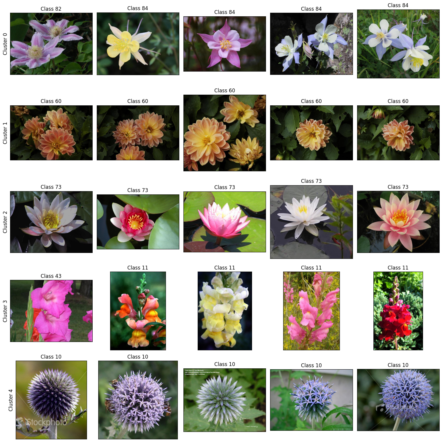
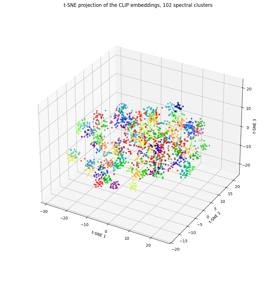
Inspect the clusters: the first images of a few clusters and a 3D t-SNE projection of the embeddings.
Compute RI, ARI, NMI, and interpret the results.
Repeat the clustering on the similarity matrix instead of the embeddings.

1. Setup and Load Data¶

from collections.abc import Sequence

import matplotlib.pyplot as plt
import numpy as np
import seaborn as sns
from matplotlib.axes import Axes
from sklearn.cluster import SpectralClustering
from sklearn.manifold import TSNE
from sklearn.metrics import (
    adjusted_rand_score,
    normalized_mutual_info_score,
    rand_score,
)

from pyvisim.datasets import OxfordFlowerDataset
from pyvisim.distance import cosine_similarity
from pyvisim.neural_networks import ClipEmbedder
from pyvisim.typing import FloatNumpyArray, IntNumpyArray

/home/runner/work/Python-Visual-Similarity/Python-Visual-Similarity/.venv/lib/python3.10/site-packages/tqdm/auto.py:21: TqdmWarning: IProgress not found. Please update jupyter and ipywidgets. See https://ipywidgets.readthedocs.io/en/stable/user_install.html
  from .autonotebook import tqdm as notebook_tqdm

Helpers¶

All helpers used in this notebook are defined here. The first cell clusters the features and scores the result against the ground-truth classes.

RANDOM_STATE = 42


def cluster_spectrally(features: FloatNumpyArray, n_clusters: int) -> IntNumpyArray:
    """
    Assign every row of ``features`` to one of ``n_clusters`` spectral clusters.

    :param features: Array of shape (N, D) with one feature vector per image
    :param n_clusters: Number of clusters to form
    :return: Cluster id of every image, shape (N,)
    """
    model = SpectralClustering(
        n_clusters=n_clusters, affinity="nearest_neighbors", random_state=RANDOM_STATE
    )
    return np.asarray(model.fit_predict(features))


def score_clustering(
    true_labels: IntNumpyArray, cluster_labels: IntNumpyArray
) -> dict[str, float]:
    """
    Compare a clustering against the ground-truth classes.

    :param true_labels: Ground-truth class of every image, shape (N,)
    :param cluster_labels: Cluster id of every image, shape (N,)
    :return: Rand index, adjusted Rand index and normalized mutual information
    """
    return {
        "RI": rand_score(true_labels, cluster_labels),
        "ARI": adjusted_rand_score(true_labels, cluster_labels),
        "NMI": normalized_mutual_info_score(true_labels, cluster_labels),
    }


def print_scores(scores: dict[str, float], heading: str) -> None:
    """
    Print clustering scores under a heading.

    :param scores: Scores keyed by their name, as returned by :func:`score_clustering`
    :param heading: Line printed above the scores
    """
    print(heading)
    for name, value in scores.items():
        print(f"{name}: {value:.4f}")

The next cell shows the first images that were assigned to a cluster, one row per cluster. Every image is titled with its ground-truth class, so a row with mixed classes reveals an impure cluster at a glance.

def show_cluster_samples(
    dataset: OxfordFlowerDataset,
    cluster_labels: IntNumpyArray,
    cluster_ids: Sequence[int],
    samples_per_cluster: int,
) -> None:
    """
    Show the first images assigned to each cluster, one row per cluster.

    :param dataset: Dataset the clustering was computed on
    :param cluster_labels: Cluster id of every image in ``dataset``, shape (N,)
    :param cluster_ids: Clusters to show, in row order
    :param samples_per_cluster: Number of images per row
    """
    _, axes = plt.subplots(
        len(cluster_ids),
        samples_per_cluster,
        figsize=(3 * samples_per_cluster, 3 * len(cluster_ids)),
        squeeze=False,
    )
    for row, cluster_id in zip(axes.tolist(), cluster_ids, strict=True):
        members = np.flatnonzero(cluster_labels == cluster_id)[:samples_per_cluster]
        draw_cluster_row(row, dataset, members, cluster_id)
    plt.tight_layout()
    plt.show()


def draw_cluster_row(
    row: Sequence[Axes],
    dataset: OxfordFlowerDataset,
    members: IntNumpyArray,
    cluster_id: int,
) -> None:
    """
    Draw the images of one cluster onto a row of axes.

    Axes left over when the cluster has fewer members than the row has axes
    are hidden.

    :param row: Axes of the row, one per image
    :param dataset: Dataset the images are read from
    :param members: Indices into ``dataset`` of the images to draw
    :param cluster_id: Cluster the images belong to, shown as the row label
    """
    for axis, index in zip(row, members, strict=False):
        image, label, _ = dataset[index]
        axis.imshow(image)
        axis.set_title(f"Class {label}")
    for axis in row[len(members) :]:
        axis.set_visible(False)
    for axis in row:
        axis.set_xticks([])
        axis.set_yticks([])
    row[0].set_ylabel(f"Cluster {cluster_id}", fontsize=12)

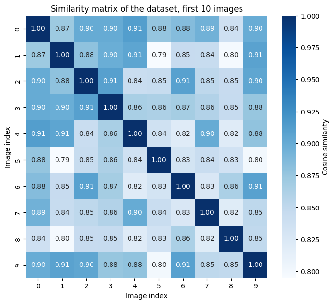
The last two helpers plot data: a 3D t-SNE projection of the embeddings, in which every cluster gets its own colour, and an annotated heatmap of a similarity matrix.

def project_to_3d(features: FloatNumpyArray) -> FloatNumpyArray:
    """
    Project feature vectors to three dimensions with t-SNE.

    :param features: Array of shape (N, D)
    :return: Array of shape (N, 3)
    """
    return TSNE(n_components=3, perplexity=40, random_state=RANDOM_STATE).fit_transform(features)


def plot_clusters_3d(
    points: FloatNumpyArray,
    cluster_labels: IntNumpyArray,
    title: str,
    colormap_name: str = "nipy_spectral",
) -> None:
    """
    Scatter 3D points, colouring the points of a cluster with the same colour.

    :param points: Array of shape (N, 3)
    :param cluster_labels: Cluster id of every point, shape (N,)
    :param title: Title of the plot
    :param colormap_name: Colormap the cluster palette is sampled from
    """
    unique_labels, dense_indices = np.unique(cluster_labels, return_inverse=True)
    cluster_count = unique_labels.size

    # Skip the colormap extremes: they are black/near-white in spectral maps.
    palette = plt.get_cmap(colormap_name)(np.linspace(0.05, 0.95, cluster_count))
    stride = np.concatenate(
        [np.arange(0, cluster_count, 2), np.arange(1, cluster_count, 2)]
    )
    colours = palette[stride][dense_indices]
    colours[cluster_labels < 0] = (0.65, 0.65, 0.65, 0.35)

    axis = plt.figure(figsize=(10, 10)).add_subplot(projection="3d")
    axis.set_box_aspect(None, zoom=0.85)
    axis.scatter(points[:, 0], points[:, 1], points[:, 2], c=colours, s=10)
    axis.set_title(title)
    axis.set_xlabel("t-SNE 1")
    axis.set_ylabel("t-SNE 2")
    axis.set_zlabel("t-SNE 3")
    plt.tight_layout()
    plt.show()


def show_similarity_heatmap(matrix: FloatNumpyArray, title: str) -> None:
    """
    Draw an annotated heatmap of a similarity matrix.

    :param matrix: Square array of pairwise similarities
    :param title: Title of the plot
    """
    plt.figure(figsize=(8, 7))
    sns.heatmap(
        matrix,
        annot=True,
        fmt=".2f",
        cmap="Blues",
        cbar_kws={"label": "Cosine similarity"},
    )
    plt.title(title)
    plt.xlabel("Image index")
    plt.ylabel("Image index")
    plt.show()

Load the validation and test datasets.¶

dataset = OxfordFlowerDataset(purpose=["validation", "test"])
true_labels = np.array(dataset.labels)
print("Number of images in the dataset:", len(dataset))

Downloading labels.mat:   0%|          | 0.00/502 [00:00<?, ?B/s]

Downloading labels.mat: 100%|██████████| 502/502 [00:00<00:00, 1.58MB/s]

Downloading setid.mat:   0%|          | 0.00/15.0k [00:00<?, ?B/s]

Downloading setid.mat: 100%|██████████| 15.0k/15.0k [00:00<00:00, 43.8MB/s]

Downloading images.tgz:   0%|          | 0.00/345M [00:00<?, ?B/s]

Downloading images.tgz:   0%|          | 32.8k/345M [00:00<18:17, 314kB/s]

Downloading images.tgz:   0%|          | 98.3k/345M [00:00<11:46, 488kB/s]

Downloading images.tgz:   0%|          | 180k/345M [00:00<09:23, 612kB/s]

Downloading images.tgz:   0%|          | 295k/345M [00:00<07:16, 789kB/s]

Downloading images.tgz:   0%|          | 426k/345M [00:00<06:05, 943kB/s]

Downloading images.tgz:   0%|          | 590k/345M [00:00<05:02, 1.14MB/s]

Downloading images.tgz:   0%|          | 770k/345M [00:00<04:22, 1.31MB/s]

Downloading images.tgz:   0%|          | 1.06M/345M [00:00<03:16, 1.75MB/s]

Downloading images.tgz:   0%|          | 1.41M/345M [00:00<02:36, 2.20MB/s]

Downloading images.tgz:   1%|          | 1.95M/345M [00:01<01:51, 3.08MB/s]

Downloading images.tgz:   1%|          | 2.52M/345M [00:01<01:31, 3.74MB/s]

Downloading images.tgz:   1%|          | 3.62M/345M [00:01<01:00, 5.68MB/s]

Downloading images.tgz:   1%|▏         | 4.70M/345M [00:01<00:48, 6.99MB/s]

Downloading images.tgz:   2%|▏         | 6.88M/345M [00:01<00:30, 11.1MB/s]

Downloading images.tgz:   3%|▎         | 8.95M/345M [00:01<00:24, 13.5MB/s]

Downloading images.tgz:   4%|▎         | 12.5M/345M [00:01<00:17, 19.0MB/s]

Downloading images.tgz:   5%|▍         | 16.1M/345M [00:01<00:14, 23.0MB/s]

Downloading images.tgz:   6%|▌         | 20.1M/345M [00:01<00:12, 26.7MB/s]

Downloading images.tgz:   7%|▋         | 24.1M/345M [00:02<00:10, 29.3MB/s]

Downloading images.tgz:   8%|▊         | 28.1M/345M [00:02<00:10, 31.1MB/s]

Downloading images.tgz:   9%|▉         | 32.2M/345M [00:02<00:09, 32.4MB/s]

Downloading images.tgz:  10%|█         | 36.2M/345M [00:02<00:09, 33.1MB/s]

Downloading images.tgz:  12%|█▏        | 40.1M/345M [00:02<00:09, 33.6MB/s]

Downloading images.tgz:  13%|█▎        | 44.1M/345M [00:02<00:08, 34.1MB/s]

Downloading images.tgz:  14%|█▍        | 48.2M/345M [00:02<00:08, 34.5MB/s]

Downloading images.tgz:  15%|█▌        | 52.2M/345M [00:02<00:08, 34.6MB/s]

Downloading images.tgz:  16%|█▋        | 56.1M/345M [00:02<00:08, 34.7MB/s]

Downloading images.tgz:  17%|█▋        | 60.2M/345M [00:03<00:08, 34.8MB/s]

Downloading images.tgz:  19%|█▊        | 64.2M/345M [00:03<00:08, 34.9MB/s]

Downloading images.tgz:  20%|█▉        | 68.2M/345M [00:03<00:07, 35.0MB/s]

Downloading images.tgz:  21%|██        | 72.2M/345M [00:03<00:07, 34.9MB/s]

Downloading images.tgz:  22%|██▏       | 76.2M/345M [00:03<00:07, 35.0MB/s]

Downloading images.tgz:  23%|██▎       | 80.2M/345M [00:03<00:07, 34.9MB/s]

Downloading images.tgz:  24%|██▍       | 84.2M/345M [00:03<00:07, 35.0MB/s]

Downloading images.tgz:  26%|██▌       | 88.2M/345M [00:03<00:07, 35.1MB/s]

Downloading images.tgz:  27%|██▋       | 92.2M/345M [00:04<00:07, 35.1MB/s]

Downloading images.tgz:  28%|██▊       | 96.2M/345M [00:04<00:07, 35.1MB/s]

Downloading images.tgz:  29%|██▉       | 100M/345M [00:04<00:06, 35.0MB/s] 

Downloading images.tgz:  30%|███       | 104M/345M [00:04<00:06, 35.0MB/s]

Downloading images.tgz:  31%|███▏      | 108M/345M [00:04<00:06, 35.1MB/s]

Downloading images.tgz:  33%|███▎      | 112M/345M [00:04<00:06, 35.1MB/s]

Downloading images.tgz:  34%|███▎      | 116M/345M [00:04<00:06, 35.1MB/s]

Downloading images.tgz:  35%|███▍      | 120M/345M [00:04<00:06, 35.1MB/s]

Downloading images.tgz:  36%|███▌      | 124M/345M [00:04<00:06, 35.0MB/s]

Downloading images.tgz:  37%|███▋      | 128M/345M [00:05<00:06, 35.1MB/s]

Downloading images.tgz:  38%|███▊      | 132M/345M [00:05<00:06, 35.0MB/s]

Downloading images.tgz:  40%|███▉      | 136M/345M [00:05<00:05, 35.0MB/s]

Downloading images.tgz:  41%|████      | 140M/345M [00:05<00:05, 35.0MB/s]

Downloading images.tgz:  42%|████▏     | 144M/345M [00:05<00:05, 35.0MB/s]

Downloading images.tgz:  43%|████▎     | 148M/345M [00:05<00:05, 35.0MB/s]

Downloading images.tgz:  44%|████▍     | 152M/345M [00:05<00:05, 35.0MB/s]

Downloading images.tgz:  45%|████▌     | 156M/345M [00:05<00:05, 35.0MB/s]

Downloading images.tgz:  46%|████▋     | 160M/345M [00:05<00:05, 34.9MB/s]

Downloading images.tgz:  48%|████▊     | 164M/345M [00:06<00:05, 35.0MB/s]

Downloading images.tgz:  49%|████▉     | 168M/345M [00:06<00:05, 35.0MB/s]

Downloading images.tgz:  50%|████▉     | 172M/345M [00:06<00:04, 35.0MB/s]

Downloading images.tgz:  51%|█████     | 176M/345M [00:06<00:04, 35.1MB/s]

Downloading images.tgz:  52%|█████▏    | 180M/345M [00:06<00:04, 35.1MB/s]

Downloading images.tgz:  53%|█████▎    | 184M/345M [00:06<00:04, 35.0MB/s]

Downloading images.tgz:  55%|█████▍    | 188M/345M [00:06<00:04, 35.1MB/s]

Downloading images.tgz:  56%|█████▌    | 192M/345M [00:06<00:04, 35.2MB/s]

Downloading images.tgz:  57%|█████▋    | 196M/345M [00:06<00:04, 35.1MB/s]

Downloading images.tgz:  58%|█████▊    | 200M/345M [00:07<00:04, 35.0MB/s]

Downloading images.tgz:  59%|█████▉    | 204M/345M [00:07<00:04, 35.0MB/s]

Downloading images.tgz:  60%|██████    | 208M/345M [00:07<00:03, 35.0MB/s]

Downloading images.tgz:  62%|██████▏   | 212M/345M [00:07<00:03, 35.1MB/s]

Downloading images.tgz:  63%|██████▎   | 216M/345M [00:07<00:03, 35.0MB/s]

Downloading images.tgz:  64%|██████▍   | 220M/345M [00:07<00:03, 35.1MB/s]

Downloading images.tgz:  65%|██████▌   | 224M/345M [00:07<00:03, 35.0MB/s]

Downloading images.tgz:  66%|██████▌   | 228M/345M [00:07<00:03, 35.0MB/s]

Downloading images.tgz:  67%|██████▋   | 232M/345M [00:08<00:03, 35.1MB/s]

Downloading images.tgz:  68%|██████▊   | 236M/345M [00:08<00:03, 34.9MB/s]

Downloading images.tgz:  70%|██████▉   | 240M/345M [00:08<00:02, 35.0MB/s]

Downloading images.tgz:  71%|███████   | 244M/345M [00:08<00:02, 35.1MB/s]

Downloading images.tgz:  72%|███████▏  | 248M/345M [00:08<00:02, 35.1MB/s]

Downloading images.tgz:  73%|███████▎  | 252M/345M [00:08<00:02, 35.1MB/s]

Downloading images.tgz:  74%|███████▍  | 256M/345M [00:08<00:02, 35.1MB/s]

Downloading images.tgz:  75%|███████▌  | 260M/345M [00:08<00:02, 35.0MB/s]

Downloading images.tgz:  77%|███████▋  | 264M/345M [00:08<00:02, 35.1MB/s]

Downloading images.tgz:  78%|███████▊  | 268M/345M [00:09<00:02, 35.1MB/s]

Downloading images.tgz:  79%|███████▉  | 272M/345M [00:09<00:02, 35.0MB/s]

Downloading images.tgz:  80%|████████  | 276M/345M [00:09<00:01, 35.0MB/s]

Downloading images.tgz:  81%|████████▏ | 280M/345M [00:09<00:01, 35.0MB/s]

Downloading images.tgz:  82%|████████▏ | 284M/345M [00:09<00:01, 35.1MB/s]

Downloading images.tgz:  84%|████████▎ | 288M/345M [00:09<00:01, 35.1MB/s]

Downloading images.tgz:  85%|████████▍ | 292M/345M [00:09<00:01, 35.2MB/s]

Downloading images.tgz:  86%|████████▌ | 296M/345M [00:09<00:01, 35.1MB/s]

Downloading images.tgz:  87%|████████▋ | 300M/345M [00:09<00:01, 35.2MB/s]

Downloading images.tgz:  88%|████████▊ | 304M/345M [00:10<00:01, 35.2MB/s]

Downloading images.tgz:  89%|████████▉ | 308M/345M [00:10<00:01, 35.2MB/s]

Downloading images.tgz:  91%|█████████ | 312M/345M [00:10<00:00, 35.1MB/s]

Downloading images.tgz:  92%|█████████▏| 316M/345M [00:10<00:00, 34.8MB/s]

Downloading images.tgz:  93%|█████████▎| 320M/345M [00:10<00:00, 35.1MB/s]

Downloading images.tgz:  94%|█████████▍| 324M/345M [00:10<00:00, 35.1MB/s]

Downloading images.tgz:  95%|█████████▌| 328M/345M [00:10<00:00, 35.1MB/s]

Downloading images.tgz:  96%|█████████▋| 332M/345M [00:10<00:00, 35.2MB/s]

Downloading images.tgz:  98%|█████████▊| 336M/345M [00:10<00:00, 35.1MB/s]

Downloading images.tgz:  99%|█████████▊| 340M/345M [00:11<00:00, 34.9MB/s]

Downloading images.tgz: 100%|█████████▉| 344M/345M [00:11<00:00, 35.0MB/s]

Downloading images.tgz: 100%|██████████| 345M/345M [00:11<00:00, 30.8MB/s]

Extracting images.tgz:   0%|          | 0/8190 [00:00<?, ?file/s]

Extracting images.tgz:   6%|▌         | 470/8190 [00:00<00:01, 4688.28file/s]

Extracting images.tgz:  12%|█▏        | 946/8190 [00:00<00:01, 4725.85file/s]

Extracting images.tgz:  17%|█▋        | 1419/8190 [00:00<00:01, 4718.06file/s]

Extracting images.tgz:  23%|██▎       | 1891/8190 [00:00<00:01, 4613.58file/s]

Extracting images.tgz:  29%|██▉       | 2361/8190 [00:00<00:01, 4642.69file/s]

Extracting images.tgz:  35%|███▍      | 2826/8190 [00:00<00:01, 4631.56file/s]

Extracting images.tgz:  40%|████      | 3290/8190 [00:00<00:01, 4598.65file/s]

Extracting images.tgz:  46%|████▌     | 3750/8190 [00:00<00:00, 4565.79file/s]

Extracting images.tgz:  52%|█████▏    | 4222/8190 [00:00<00:00, 4612.33file/s]

Extracting images.tgz:  58%|█████▊    | 4729/8190 [00:01<00:00, 4752.20file/s]

Extracting images.tgz:  64%|██████▍   | 5231/8190 [00:01<00:00, 4830.80file/s]

Extracting images.tgz:  70%|██████▉   | 5728/8190 [00:01<00:00, 4870.53file/s]

Extracting images.tgz:  76%|███████▌  | 6225/8190 [00:01<00:00, 4898.19file/s]

Extracting images.tgz:  82%|████████▏ | 6727/8190 [00:01<00:00, 4934.48file/s]

Extracting images.tgz:  88%|████████▊ | 7221/8190 [00:01<00:00, 4876.63file/s]

Extracting images.tgz:  94%|█████████▍| 7724/8190 [00:01<00:00, 4921.59file/s]

Extracting images.tgz: 100%|██████████| 8190/8190 [00:01<00:00, 4791.19file/s]

Number of images in the dataset: 2040

2. Compute CLIP embeddings¶

Define the CLIP embedder¶

clip_embedder = ClipEmbedder(variant="ViT-B/32", pretrained="openai")

Compute the CLIP embeddings for both the validation and test splits¶

clip_embeddings = clip_embedder.embed(image for image, *_ in dataset)

3. Cluster into 102 Clusters¶

102 is the number of classes in the Oxford Flowers dataset. We want to see how well the clustering algorithm can cluster the images into these classes.

NUM_CLASSES = 102
cluster_labels = cluster_spectrally(clip_embeddings, n_clusters=NUM_CLASSES)

Inspect the clusters¶

Before looking at any score, let’s look at the clusters themselves. The grid below shows the first 5 images of each of the first 5 clusters. Ideally, all images in a row share the same class.

show_cluster_samples(
    dataset, cluster_labels, cluster_ids=range(5), samples_per_cluster=5
)

../../_images/b20e5cfe8b041c41ab61cc51ae487ef89782e574abbbe12ce4359bea9472e181.png

Visualize the embeddings in 3D¶

t-SNE is used to project the 512-dimensional CLIP embeddings onto three dimensions.

projected_embeddings = project_to_3d(clip_embeddings)
plot_clusters_3d(
    projected_embeddings,
    cluster_labels,
    title=f"t-SNE projection of the CLIP embeddings, {NUM_CLASSES} spectral clusters",
)

../../_images/9bb49fda286352cf4da2539f22ea5d0a825c4fd139c84322ba7df4a678a44c93.png

Compute RI, ARI, NMI¶

The Rand index (RI) is the fraction of image pairs on which the clustering and the ground truth agree. The adjusted Rand index (ARI) corrects it for chance agreement, and the normalized mutual information (NMI) measures how much knowing the cluster of an image tells us about its class.

scores = score_clustering(true_labels, cluster_labels)
heading = f"Spectral clustering of the embeddings into {NUM_CLASSES} clusters:"
print_scores(scores, heading)

Spectral clustering of the embeddings into 102 clusters:
RI: 0.9912
ARI: 0.6133
NMI: 0.8931

4. Cluster on the Similarity Matrix¶

Now, instead of using the embeddings themselves, we will use the similarity matrix of the embeddings to cluster the images. So each row in this matrix will represent the similarity of an image to all other images in the dataset (hence, all diagonal elements will be 1).

similarity_matrix = cosine_similarity(clip_embeddings, clip_embeddings)
show_similarity_heatmap(
    similarity_matrix[:10, :10],
    title="Similarity matrix of the dataset, first 10 images",
)

../../_images/e99667bb380e001afca9665d7d761303baa5b9a79fa29c8f4ce81a0a5809e49d.png

similarity_cluster_labels = cluster_spectrally(
    similarity_matrix, n_clusters=NUM_CLASSES
)
similarity_scores = score_clustering(true_labels, similarity_cluster_labels)
heading = f"Spectral clustering of the similarity matrix into {NUM_CLASSES} clusters:"
print_scores(similarity_scores, heading)

/home/runner/work/Python-Visual-Similarity/Python-Visual-Similarity/.venv/lib/python3.10/site-packages/sklearn/cluster/_spectral.py:706: UserWarning: The spectral clustering API has changed. ``fit``now constructs an affinity matrix from data. To use a custom affinity matrix, set ``affinity=precomputed``.
  warnings.warn(

Spectral clustering of the similarity matrix into 102 clusters:
RI: 0.9884
ARI: 0.4214
NMI: 0.7676

5. Conclusion¶

We’ve demonstrated:

How to cluster images directly on CLIP embeddings.
How to inspect the clusters visually, through sample images and a 3D t-SNE projection.
How to compute RI, ARI and NMI for objective evaluation.

For CLIP, clustering on the embeddings themselves performs significantly better than clustering on the similarity matrix.