2.2 Pipeline with Deep Features
In this notebook, we’ll:
Load (or extract) deep features from a set of images (Oxford Flowers or any dataset).
Train a single KMeans and GMM model (both with 32 clusters/components).
Set up a VLAD embedder using the KMeans model.
Set up a Fisher Vector embedder using the GMM model.
Use each embedder separately for retrieval, then combine them in a pipeline, and compare retrieval metrics.
For more detail, see the paper below.
Reference:
[1]Weixia Zhang, Jia Yan, Wenxuan Shi, Tianpeng Feng, and Dexiang Deng, “Refining Deep Convolutional Features for Improving Fine-Grained Image Recognition,” EURASIP Journal on Image and Video Processing, 2017.
import os
from typing import Any

import matplotlib.pyplot as plt
import numpy as np
import seaborn as sns
import torch

from pyvisim.distance import cosine_similarity
from pyvisim.classic import FisherVectorEmbedder, Pipeline, VLADEmbedder
from pyvisim.datasets import OxfordFlowerDataset  # or any dataset you have
from pyvisim.neural_networks.features import DeepConvFeature
from pyvisim.retrieval.image_store import InMemoryImageEmbeddingStore
from pyvisim.typing import NumpyArray, UInt8NumpyArray
/home/runner/work/Python-Visual-Similarity/Python-Visual-Similarity/.venv/lib/python3.10/site-packages/tqdm/auto.py:21: TqdmWarning: IProgress not found. Please update jupyter and ipywidgets. See https://ipywidgets.readthedocs.io/en/stable/user_install.html
  from .autonotebook import tqdm as notebook_tqdm
Helper functions
def plot_image(image: UInt8NumpyArray | torch.Tensor, title: str = "Image") -> None:
    """
    Plot a single image.

    :param image: Image as a NumPy array (H, W, C) or torch tensor (C, H, W)
    :param title: Title of the plot
    """
    plt.figure(figsize=(10, 10))
    if isinstance(image, torch.Tensor):
        image = image.detach().cpu()
        if image.ndim == 3:
            image = image.permute(1, 2, 0)
        image = image.numpy()
    plt.imshow(image)
    plt.axis("off")
    plt.title(title)
    plt.show()


def plot_and_save_heatmap(
    matrix: list[Any] | NumpyArray | torch.Tensor,
    figsize: tuple[int, int] | None = None,
    x_tick_labels: list[str] | None = None,
    y_tick_labels: list[str] | None = None,
    cbar_kws: dict[str, str] | None = None,
    title: str = "Heatmap",
    x_label: str = "X Axis",
    y_label: str = "Y Axis",
    show: bool = True,
    save_fig_path: str | None = None,
) -> None:
    """
    Plot a heatmap using the specified matrix.

    :param matrix: matrix
    :param figsize: figure size
    :param x_tick_labels: x-axis tick labels
    :param y_tick_labels: y-axis tick labels
    :param cbar_kws: colorbar keyword arguments
    :param title: title of the plot
    :param x_label: x-axis label
    :param y_label: y-axis label
    :param show: whether to display the plot
    :param save_fig_path: Path to save the figure
    """
    if isinstance(matrix, list):
        matrix = np.array(matrix)
    elif isinstance(matrix, torch.Tensor):
        matrix = matrix.detach().cpu().numpy()

    figsize = (
        (
            int(matrix.shape[1] * 0.7),
            int(matrix.shape[0] * 0.7),
        )
        if figsize is None
        else figsize
    )
    plt.figure(figsize=figsize)
    sns.heatmap(
        matrix,
        annot=True,
        fmt=".2f",
        cmap="viridis",
        xticklabels=x_tick_labels if x_tick_labels else list(range(matrix.shape[1])),
        yticklabels=y_tick_labels if y_tick_labels else list(range(matrix.shape[0])),
        cbar_kws=cbar_kws if cbar_kws else {"label": "value"},
    )
    plt.title(title)
    plt.xlabel(x_label)
    plt.ylabel(y_label)
    if save_fig_path:
        plt.savefig(save_fig_path)
    if show:
        plt.show()
    plt.close()
1. Load Dataset and Extract Deep Features
We’ll load a subset of images and collect their deep descriptors.
train_dataset = OxfordFlowerDataset(
    purpose="train",
)
Let’s define our deep extractor
extractor = DeepConvFeature(
    backbone="resnet18",
    layer_index=-1,
)
Downloading: "https://download.pytorch.org/models/resnet18-f37072fd.pth" to /home/runner/work/Python-Visual-Similarity/Python-Visual-Similarity/.cache/torch/hub/checkpoints/resnet18-f37072fd.pth
0%| | 0.00/44.7M [00:00<?, ?B/s]
1%| | 384k/44.7M [00:00<00:14, 3.24MB/s]
4%|▎ | 1.62M/44.7M [00:00<00:05, 7.99MB/s]
13%|█▎ | 5.88M/44.7M [00:00<00:01, 23.2MB/s]
41%|████▏ | 18.5M/44.7M [00:00<00:00, 62.4MB/s]
100%|██████████| 44.7M/44.7M [00:00<00:00, 89.7MB/s]
2. Initialize Embedders: VLAD and Fisher Vector
vlad_embedder = VLADEmbedder(
    feature_extractor=extractor,
    n_clusters=32,
    power_norm_weight=1,
)

fisher_embedder = FisherVectorEmbedder(
    feature_extractor=extractor,
    n_components=32,
    power_norm_weight=0.5,
)
Train the KMeans and GMM models
Both models are trained on the deep features of every IMAGE_STEP-th training image. The training split is sorted by class, so the step keeps all 102 classes represented. Set it to 1 to train on the whole training split, which takes quite a bit of time. For the Fisher Vector, the feature dimension is reduced by half using PCA first.
IMAGE_STEP = 12
train_indices = range(0, len(train_dataset), IMAGE_STEP)
print(f"Training on {len(train_indices)} images")

vlad_embedder.learn(train_dataset[i][0] for i in train_indices)
fisher_embedder.learn(
    (train_dataset[i][0] for i in train_indices),
    dim_reduction_factor=2,
)
/home/runner/work/Python-Visual-Similarity/Python-Visual-Similarity/.venv/lib/python3.10/site-packages/torchvision/transforms/functional.py:154: UserWarning: The given NumPy array is not writable, and PyTorch does not support non-writable tensors. This means writing to this tensor will result in undefined behavior. You may want to copy the array to protect its data or make it writable before converting it to a tensor. This type of warning will be suppressed for the rest of this program. (Triggered internally at /__w/pytorch/pytorch/torch/csrc/utils/tensor_numpy.cpp:213.)
  img = torch.from_numpy(pic.transpose((2, 0, 1))).contiguous()
Training on 513 images
[INFO] Learning the visual vocabulary with the following parameters:
   - Number of clusters: 32
   - Feature Extractor used: DeepConvFeature
   - Dimension of the feature space: 512
[INFO] Learning the visual vocabulary with the following parameters:
   - Number of clusters: 32
   - Feature Extractor used: DeepConvFeature
   - Dimension of the feature space: 512
- New dimension after PCA reduction: 256
/home/runner/work/Python-Visual-Similarity/Python-Visual-Similarity/pyvisim/classic/_base_embedder.py:436: FutureWarning: Best of 1 EM run(s) did not converge within 100 iterations; consider raising max_iter, raising tol or increasing n_init.
  self._clustering_model.fit(features)
4. Compute vectors
Select images for comparison
image1, *_ = train_dataset[0]
image2, *_ = train_dataset[1]
plot_image(image1)
plot_image(image2)
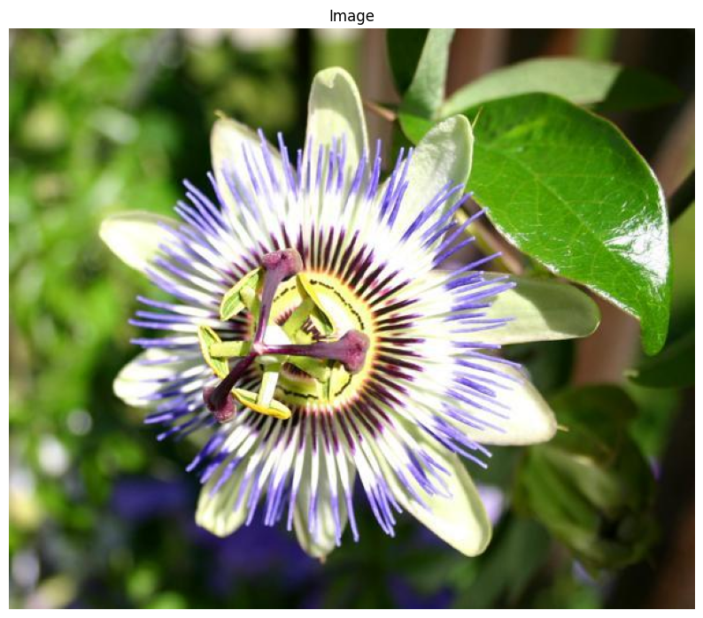
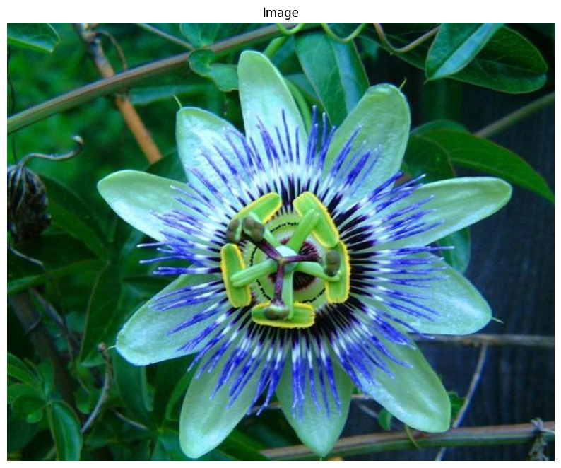
Compute VLAD and Fisher Vectors
fisher_vector_1 = fisher_embedder.embed(image1)
vlad_vector_1 = vlad_embedder.embed(image1)
print(
    f"Shape of Fisher Vector: {fisher_vector_1.shape}, Shape of VLAD Vector: {vlad_vector_1.shape}"
)

fisher_vector_2 = fisher_embedder.embed(image2)
vlad_vector_2 = vlad_embedder.embed(image2)
Shape of Fisher Vector: (1, 16416), Shape of VLAD Vector: (1, 16384)
Compute similarity scores using VLAD and Fisher Vectors
print("Cosine similarity using VLAD:", vlad_embedder.similarity_score(image1, image2))
print(
    "Cosine similarity using Fisher Vectors:",
    fisher_embedder.similarity_score(image1, image2),
)
Cosine similarity using VLAD: [[0.22199482]]
Cosine similarity using Fisher Vectors: [[0.11918212]]
Use a Pipeline
We can combine both steps above by using the pipeline class.
pipeline = Pipeline([vlad_embedder, fisher_embedder])
Compare images using the pipeline
The result is the similarity score of the concatenated VLAD and Fisher vectors.
sim_score = pipeline.similarity_score(image1, image2)
print("Scores using the pipeline:", sim_score)
Scores using the pipeline: [[0.17058846]]
This is equal to:
combined_vector_1 = np.hstack((vlad_vector_1, fisher_vector_1))
combined_vector_2 = np.hstack((vlad_vector_2, fisher_vector_2))
print(
    "Cosine similarity using concatenated vectors:",
    cosine_similarity(combined_vector_1, combined_vector_2),
)  # Cosine similarity was chosen as `similarity_func` for the embedders
Cosine similarity using concatenated vectors: [[0.17058847]]
You can also compare two batches of images at once. The shape is the similarity matrix of size (batch_1_size, batch_2_size).
batch_1 = (train_dataset[i][0] for i in range(5))
batch_2 = (train_dataset[i][0] for i in range(5, 15))
similarity_matrix = pipeline.similarity_score(batch_1, batch_2)
plot_and_save_heatmap(
    similarity_matrix,
    x_tick_labels=[f"Image {i}" for i in range(10)],
    y_tick_labels=[f"Image {i}" for i in range(5)],
    figsize=(10, 5),
)
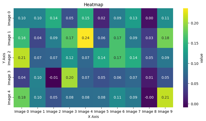
You can call the embed method, just like with VLADEmbedder and FisherVectorEmbedder. Each image is embedded using the embedders in the pipeline, and the end result is the concatenation of the vectors.
images_1_5 = [train_dataset[i][0] for i in range(5)]
embedding = pipeline.embed(images_1_5)
print("Shape of embedded batch:", embedding.shape)  # (num_images, dim_vlad + dim_fisher)
Shape of embedded batch: (5, 32800)
Build an image store
The store embeds the images with the pipeline. Its paths are the image paths and its embeddings are the concatenated VLAD and Fisher vectors, L2-normalised since the store is built in the cosine space.
image_paths = train_dataset.image_paths[:5]
store = InMemoryImageEmbeddingStore(image_paths=image_paths, embedder=pipeline)
store.build_store()
{
    os.path.basename(path): vector
    for path, vector in zip(store.paths, store.embeddings, strict=True)
}
{'image_00001.jpg': array([ 0.        ,  0.        ,  0.        , ..., -0.01389456,
         0.00925594, -0.01364283], shape=(32800,), dtype=float32),
 'image_00002.jpg': array([ 0.        ,  0.        ,  0.        , ...,  0.00588449,
        -0.00999607,  0.00411336], shape=(32800,), dtype=float32),
 'image_00003.jpg': array([-0.00975044,  0.00835862,  0.00189669, ...,  0.00781672,
         0.00320898,  0.00404138], shape=(32800,), dtype=float32),
 'image_00004.jpg': array([-0.00307262, -0.00683291, -0.00322677, ...,  0.00445038,
         0.00297608,  0.00357034], shape=(32800,), dtype=float32),
 'image_00005.jpg': array([ 0.        ,  0.        ,  0.        , ...,  0.00565641,
        -0.01162751,  0.00823683], shape=(32800,), dtype=float32)}
Print the pipeline to see the embedders it contains.
print(pipeline)
Pipeline(
embedders=[VLADEmbedder(feature_extractor=DeepConvFeature,
similarity_func=cosine,
Number of cluster=32,
Power Norm Weight=1,
Norm Order=2)
FisherVectorEmbedder(feature_extractor=DeepConvFeature,
similarity_func=cosine,
Number of cluster=32,
Power Norm Weight=0.5,
Norm Order=2)],
similarity_func=cosine)